Memory and Computation Cost of Large Language Models

I have recently started following/auditing Stanford’s CS336 course, and while going through the second lecture I took some notes which I think can be also valuable for others.. This lecture focuses on analysing the computation and memory cost of LLMs, with explanations. To understand them better, you also need to understand the computation graphs a little bit, which I added as an interlude from Andreas Geiger’s notes on the topic. Furthermore, I reiterated the OpenAI’s analysis on the memory and compute requirements, while trying to explain the reasoning.

Motivating Questions

How long would it take to train a 70B parameter model on 15T tokens on 1024 H100s?

Determine the total number of FLOPs you need
Get the FLOPs per second from the info sheet (H100: 1979e12 / 2)
Get model flops utilization -> A metric to measure efficiency of your training
Flops you can use per day: GPU Flops Capacity x Model Flops Utilization x Number of GPUs x Seconds in a Day
Then, the training will take “Needed number of FLOPs / FLOPS you can use per day” days.

What is the largest model that you can train on 8 H100s using AdamW (naively)?

Get the VRAM size of the GPU in bytes
Calculate the bytes you need per parameter (Depends on the precision you use and the optimizer)
Then, simply divide to find the biggest model you can train within the constraints

Note: This does not account for the cost of activations, which depend on the batch size and the sequence length.

Memory Accounting

Tensors are the basic building blocks for everything else.
Creating tensors without initializing values:

x = torch.empty(4, 8) # Create an empty 4, 8 matrix
nn.init.trunc_normal_(x, mean=0, std=1, a=-2, b=2) # Initialize the values in a specific way

Most tensors are stored as floating point numbers.

Reminder about Floating Point Representations

In real life, we use scientific notation to separate the interesting parts of the number and its order of magnitude.
For example, Avogadro number: $6.022 \times 10^{23}$.
- We say this number has 4 digits of precision, and this actually represents some range of possible measurements: $[ 6.022 \times 10^{23} – \varepsilon, 6.022 \times 10^{23} + \varepsilon ]$ where $\varepsilon \approx 0.001 \times 10^{23}$. (If $\varepsilon$ were to be larger, then it would be put into the digits of precision part, so we know our error must be smaller than $\varepsilon \times 10^{23}$)
In this case, $6.022$ is called the significand (or fraction) and $23$ is called the exponent.

float32 (=fp32=Single Precision)

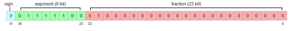
32 bits, 1 for sign, 8 for exponent and 23 bits for the fraction.
It is the default.
In deep learning, unlike scientific computing, we do not use double precision (float64).
Memory is determined by the number of values, and types of those values.
- e.g. assume a (4, 8) matrix. Its memory cost is $4 \times 8 \times 32 = 1024$ bits, or $4\times8\times4 = 128$ bytes (8 bits = 1 byte, float32 = 4 bytes)
Example: One matrix in the feedforward layer of GPT-3:
- Embedding size: 12_288
- Matrix size: (12_288 * 4, 12_288)
- This means this matrix in single precision would cost 2306 MB, or 2.25 GB.
Maximum positive number you can represent: $\underbrace{(1 + \underbrace{8388607/8388608}_{\text{Fraction}})}_{\text{Mantissa}} \times 2^{127}$ (127 because half is used for the negative representation, and the upper and lower ends are reserved for special representations like 0, nan, infinity).
Notice how precise you can get, and range is given by the exponent bits.

float16 (=fp16=Half Precision)

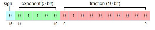
16 bits, 1 sign, 5 exponent, 10 fraction.
Cuts the memory usage in half.
However, it is not great for small numbers, as e.g. 1e-8 would go to $0$
This can lead to underflows in gradient if used during training.
Maximum positive number you can represent: $\underbrace{(1 + \underbrace{1023/1024}_{\text{Fraction}})}_{\text{Mantissa}} \times 2^{15}$
Now, our mantissa is less precise, and our range is also smaller due to having less bits for exponents

bfloat16 (Brain Floating Point)

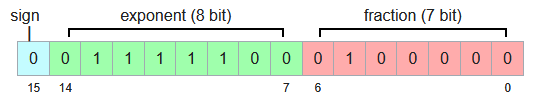
For deep learning, we care about the dynamic range more then we care about the fraction bit because we want to have more stable gradients.
Resolution is worse (fraction/significand can be represented with 7 bits), but it has the same dynamic range as the float32 while using half the space.
Developed by Google Brain
Maximum number you can represent: $\underbrace{(1 + \underbrace{127/128}_{\text{Fraction}})}_{\text{Mantissa}} \times 2^{127}$
Notice that our mantissa is more crude, but our range is as high as fp32 again.

fp8

Standardized in 2022
Only supported by H100 and later
There are two types:
- FP8 E4M3 (exponent 4, mantissa 3)
  - Cannot represent infinities, only NAN is defined
  - This increases the range of representable numbers
  - Maximum representable number: $(1 + 6/8) \times 2^8 = 448$
    - Because they decided not to make infinities representable, they increased dynamic range
    - Because NaN is defined as all bits set to 1, you cannot represent $1+7/8 \times 2^8$.
- FP8 E5M2 (exponent 5, mantissa 2)
  - Can represent infinities and NaN
  - Maximum representable number: $(1 + 3/4) \times 2^{15} = 57,344$
Forward activations and weights require more precision, so E4M3 datatypes are best used in the forward pass.
For the backward pass, range is more important for the gradients then the precision, so E5M2 can be utilized.

Practicality

To store parameters and optimizer states, you still need float32.
- Or training can go haywire.
- fp32 -> Safe, needs more memory
- fp8, float16, bfloat16 -> Risky
- Solution: Using Mixed Precision Training!
  - e.g. some people use fp32 in attention, but bf16 for the ffns
Rule-of-thumb: Things you accumulate, you use higher precision

Compute Accounting

Tensors on GPU

Tensors get stored in CPU by default.
We need to move them to GPUs explicitly over the PCI Bus between the system memory (RAM) and the GPU memory (VRAM)

Tensor Operations

Tensor Storage

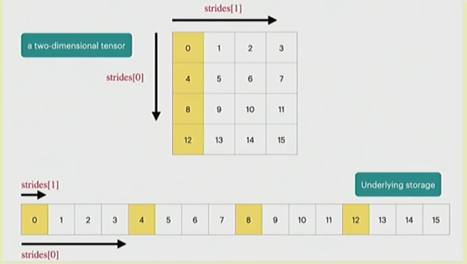
PyTorch tensors are pointers to some allocated memory with metadata describing how to get to any element of the tensor
Metadata: 1 number per dimension of the tensor
- Strides for each dimension: How many do you need to skip to get to the next element?
- In this example, strides[0] = 4 and strides[1] = 1
- To go to next row, you need to move 4 elements
- To go to the next column, you need to move 1 element
- To get to the second row, third column: ind= (1 * strides[0]) + (2 * strides[1])
  - This gives us the 4+2=6th element from the flat array
You can access this information using: x.stride(0), x.stride(1), ...

Tensor Slicing

Many operations do not create new tensors but just create new views

x = torch.tensor(
[
	[1, 2, 3],
	[4, 5, 6]
]
)

y = x[0]

print(x.untyped_storage().data_ptr() == y.untyped_storage(0).data_ptr()) # True
# (Means they point to the same place in the memory)

This includes slicing, transposing, reshaping (via view) etc.
Note: Some views are non-contiguous, so you cannot do further view operations on them.
- You can enforce it to be contiguous first:

y = x.transpose(1, 0).contiguous().view(2,3)

- But this will copy the tensor.
- Views are free, but copy’s will take additional memory and compute

Element-wise Tensor Operations

Element-wise operations always create new tensors

x = torch.tensor([1, 4, 9])
# These create new tensors
x.pow(2)
x.sqrt()
x.rsqrt()
x + x
x * 2
x / 0.5

# also
x = torch.ones(3, 3).triu() # -> Creates a new tensor (where do you keep the zeros, a new space!)

Matrix Multiplications

Usually done over batches, broadcasts etc. Some examples in the Einsum part (and what you should use instead)

Einops

Based on Einstein summation notation
Makes it easier to keep track of dimensions and do operations over different dimensions

Jaxtyping

Dimension annotations, makes it easier to use einops

x = torch.ones(2, 2, 1, 3) # batch, seq, heads, hidden

# Jaxtyping way:
x: Float[torch.Tensor, "batch seq heads hidden"] = torch.ones(2, 2, 1, 3)

Einsum

Generalized matrix multiplication

x: Float[torch.Tensor, "batch seq1 hidden"] = torch.ones(2, 3, 4)
y: Float[torch.Tensor, "batch seq2 hidden"] = torch.ones(2, 3, 4)

# Matrix multiplication over the batches:
z = x @ y.transpose(-2, -1) # batch, sequence, sequence

# Einops way of doing the same multiplication:
z = einsum(x, y, "batch seq1 hidden, batch seq2 hidden -> batch seq1 seq2")

Dimensions that are not named in the output are summed over.
Similar to slicing, you can use ... to represent “all other dimensions”:

z = einsum(x, y, "... seq1 hidden, ... seq2 hidden -> ... seq1 seq2)

Reduce

Doing aggregations over some dimensions
Works on 1 tensor

x: Float[torch.Tensor, "batch seq hidden"] = torch.ones(2, 3, 4)

# Previously, sum the hidden values:
y = x.sum(dim=-1)

# Einops:
y = reduce(x, "... hidden -> ...", "sum")

Rearrange

Sometimes, a dimension can represent two dimensions (e.g. block multiplication, some flattened views etc.)
Then, we can “rearrange” them into two dimensions again and operate on them individually if needed:

x: Float[torch.Tensor, "batch seq total_hidden"] = torch.ones(2, 3, 8)
w: Float[torch.Tensor, "hidden1 hidden2"] = torch.ones(4, 4)

x = rearrange(x, "... (heads hidden1) -> ... heads hidden1", heads=2) # dim(x) = 2, 3, 2, 4

# Operate on the hiddens
x = einsum(x, w, "... hidden1, hidden1 hidden2 -> ... hidden2")

# Arrange them back
x = rearrange(x, "... heads hidden2 -> ... (heads hidden2)")

Tensor Flops

Any basic operation like addition or multiplication is a floating-point operation (FLOP)
Confusing terminology:
- FLOPs: Floating-point operations (how much computation has been done / is being done) -> Used to quantify the computation work
- FLOP/s: Floating-point operations per second (also written as FLOPS), measures the speed of the computation being done -> Used to quantify how fast some hardware can complete computation work
Some real-life figures:
- GPT-3: 3.14e23 FLOPs
- GPT-4: 2e25 FLOPs
- A100 peak performance: 312 teraFLOP/s (312e12)
- H100 peak performance:
  - Sparse: 1979 teraFLOPs (1979e12)
  - Not-sparse: Approximately 50% of the sparse performance

Linear Model Example

We have a linear model.
We have B points.
Each point is D-dimensional.
Linear model maps each point to K outputs.

# Assume:
B = 16384
D = 32768
K = 8192

device = torch.device("cuda:0")

# Operations:
x = torch.ones(B, D, device=device)
w = torch.rand(D, K, device=device)
y = x @ w

We have one multiplication (x[i][j] * w[j][k]) and one addition per triple (i, j, k)
That means, actual number of flops is: 2 * B * D * K

(Because, e.g. check this naive implementation):

for i in range(result.shape[0]):
	    for k in range(result.shape[1]):
	        for j in range(x.shape[1]):
	            result[i][k] += x[i][j] * w[j][k]

So, for each i, j, k, we do 2 basic operations.

Other Operations

Element-wise operations on an mxn matrix requires O(m x n) FLOPs (1 basic op. per element)
Addition of two mxn matrices require m x n FLOPs (1 basic op. per element)
In general, matrix multiplication is the most expensive operation in deep learning (especially at scale)
Interpretation:
- B is the number of data points -> In transformers, tokens are the data points
- (D K) is the number of parameters
- FLOPs for forward pass is -> 2 x (# tokens) x (# parameters)
- So, this matrix multiplication “cost” generalizes to transformers (until the sequence length is too large)

Model FLOPs Utilization (MFU)

After we estimate the required FLOPs, we can measure the required wall time for a forward pass:

if torch.cuda.is_available():
	torch.cuda.synchronize()
	
def run():
	a @ b
	
	if torch.cuda.is_available():
		torch.cuda.synchronize()

num_trials = 5
total_time = timeit.timeit(run, number=num_trials)

actual_time = total_time / num_trials

Then, using the promised and estimated FLOPs for the forward pass, we can calculate the “efficiency” of our model, which is called the “Model FLOPs Utilization (MFU)”:

estimated_num_flops = 2 * B * D * K
flops_per_sec = estimated_num_flops / actual_time
promised_flops_per_sec = 67e12 # FP32 Promised flop/s for H100 (from the data sheet)
mfu = flops_per_sec/promised_flops_per_sec

MFU >= 0.5 is accepted to be good.
(For bfloat16 etc. MFU tend to be lower, even though you get speed increases. Promised FLOP/s get more “optimistic” with these data types)

Gradients – Basics

Tensor operations and calculations are relevant for the forward pass.
Gradient operations are the relevant for the backward pass.

Simple example:

$$
y = 0.5(xw – 5)^2
$$

Forward pass:

x = torch.tensor([1., 2, 3])
w = torch.tensor([1., 1, 1], requires_grad=True)
pred_y = x @ w
loss = 0.5 * (pred_y - 5).pow(2)

Backward pass:

loss.backward()
assert loss.grad is None
assert pred_y.grad is None
assert x.grad is None
assert torch.equal(w.grad, torch.tensor([1, 2, 3]))

Interlude: Computation Graphs

Minimization of a non-linear objective requires calculating the gradients $\nabla_w$.
We can efficiently compute the gradients by decomposing the computation into a sequence of atomic assignments
This sequence of atomic assignments is called a computation graph
In the forward pass, we take a training point $(x, y)$ and compute a loss

$$
\mathcal{L} = -\log p_{\text{model}}(y|x, w)
$$

Gradients $\nabla_w\mathcal{L}$ get computed during the backward pass.
Computation graphs have three kinds of nodes:
- Input Nodes
- Parameter Nodes
- Compute Nodes
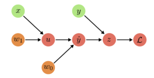
Example: Linear Regression

$u = w_1 x$
$\hat{y} = w_0 + u$
$z = \hat{y} – y$
$\mathcal{L} = z^2$

In the backward pass, goal is to find the gradients of the negative log likelihood, or in general of a loss function.
Chain Rule:

$$
\frac{d}{dx}f(g(x)) = \frac{df}{dg}\frac{dg}{dx}
$$

Multivariate Chain Rule:

$$
\frac{d}{dx}f(g_1(x), \dots, g_M(x)) = \sum_{i=1}^M \frac{\partial f}{\partial g_i} \frac{dg_i}{dx}
$$

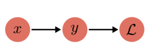
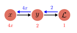
Simple example:

$y = x^2$
$\mathcal{L} = 2y$

$\to$ Loss = $2x^2$

Backward Pass:

(2)

$$
\frac{\partial \mathcal{L}}{\partial y} = \frac{\partial \mathcal{L}}{\partial \mathcal{L}} \frac{\partial \mathcal{L}}{\partial y} = 2
$$

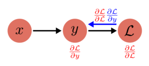
(1)

$$
\frac{\partial L}{\partial x} = \frac{\partial \mathcal{L}}{\partial{y}}\frac{\partial y}{\partial x} = \frac{\partial \mathcal{L}}{\partial y} 2x
$$

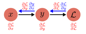
Then, when we replace the values:

$$
\frac{\partial \mathcal{L}}{\partial \mathcal{L}} = 1, \frac{\partial \mathcal{L}}{\partial \mathcal{y}} = 2 \implies \frac{\partial\mathcal{L}}{\partial y} = 1\times2 = 2
$$

$$
\frac{\partial y}{\partial x} = 2x \implies \frac{\partial\mathcal{L}}{\partial x} = 2 \times 2x = 4x
$$

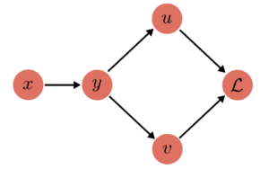
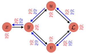
Fan-Out Example

Forward Pass:

(1) $y = y(x)$
(2) $u = u(y)$
(2) $v = v(y)$
(3) $\mathcal{L} = \mathcal{L}(u, v)$

$\to$ Loss: $\mathcal{L}\left( u(y(x)), v(y(x)) \right)$

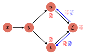
(3)

$$
\frac{\partial L}{\partial u} = \frac{\partial L}{\partial L}\frac{\partial L}{\partial u} = \frac{\partial L}{\partial u}
$$

$$
\frac{\partial L}{\partial v} = \frac{\partial L}{\partial L}\frac{\partial L}{\partial v} = \frac{\partial L}{\partial v}
$$

(2)

$$
\frac{\partial L}{\partial y} = \frac{\partial L}{\partial u}\frac{\partial u}{\partial y} + \frac{\partial L}{\partial v}\frac{\partial v}{\partial y}
$$

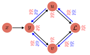
(3)

$$
\frac{\partial L}{\partial x} = \frac{\partial L}{\partial y}\frac{\partial y}{\partial x}
$$

Each computation node has 2 attributes: grad and value. PyTorch AutoGrad automatically keeps track of the operations being done, and also keeps track of the required gradient function.

This is the forward-pass:

x.value = Input
y.value = y(x.value)
u.value = u(y.value)
v.value = v(y.value)
L.value = L(u.value, v.value)

And the corresponding backward-pass:

# Initialize all the gradients
x.grad = y.grad = u.grad = v.grad = 0

# Start backward pass
L.grad = 1 
u.grad += L.grad * (L.du)(u.value, v.value) # Assume L.du is the gradient function of L wrt. u
v.grad += L.grad * (L.dv)(u.value, v.value)
y.grad += u.grad * (u.dy)(y.value)
y.grad += v.grad * (v.dy)(y.value)
x.grad += y.grad * (y.dx)(x.value)

Backprop on Tensors

So far, we talked about computation graphs for scalar values

$$
y = \sigma(w_1x + w_0)
$$

This generalizes to matrix/tensor representation as well

$$
y = \sigma(Ax + b)
$$

$A$ and $b$ have the same attributes, grad and value.
A.grad: $\nabla_A\mathcal{L}$, b.grad = $\nabla_b\mathcal{L}$
A.grad.shape == A.value.shape (Because we are measuring the “effect” of each parameter on the final loss, so we would keep track of the effect of each parameter separately)

In the first part, we already talked about implementing matrix multiplication naively with loops. Assuming here $x$ is just a data point (1D vector), and $u := Ax$:

for i in range(A.shape[0]):
	u.value[i] = 0
	for j in range(A.shape[1]):
		u.value[i] += A.value[i, j] * x.value[j]
	y.value[i] = sigmoid(u.value[i] + b.value[i])

Then, backpropagated gradients are:

For: y.value[i] = sigmoid(u.value[i] + b.value[i]

for i in range(u.value.shape[0]):
	u.grad[i] += y.grad[i] * sigmoid_grad(u.value[i] + b.value[i])
	b.grad[i] += y.grad[i] * sigmoid_grad(u.value[i] + b.value[i])

For u.value[i] += A.value[i, j] * x.value[j]:

for i in range(A.shape[0]):
	for j in range(A.shape[1]):
		A.grad[i, j] += u.grad[i] * x.value[j]
		x.grad[j] += u.grad[i] * A.value[i, j]

And when you these operations over all the batches, for grad calculation you need to sum this over all the data points in the batch.

Gradients – FLOPs

Now that we reviewed the computation graphs, we can calculate the FLOPs we need.
Assume another linear model, this time two linear transformations one after another:

x = torch.ones(B, D)
w1 = torch.randn(D, D, requires_grad=True)
w2 = torch.randn(D, K, requires_grad=True)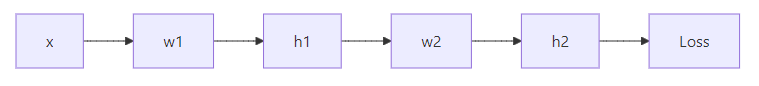

Forward FLOPs

h1 = x @ w1 # (B, D) x (D, D) -> (B, D)
h2 = h1 @ w2 # (B, D) x (D, K) -> (B, K)
loss = h2.pow(2).mean() # -> (1)

For each matrix operation, we use 2 * dim1 * dim2 * dim3 FLOPs, as established before.
In this case, first matrix operation: $2 \times B \times D \times D$
Second matrix operation: $2 \times B \times D \times K$
In total, $\text{Forward FLOPs} = (2\times B\times D\times D) + (2\times B\times D\times K)$

Backward FLOPs

h1.retain_grad()
h2.retain_grad()
loss.backward()

The loss.backward() line does all the operations we showed before. That is, model.forward() is responsible for the forward pass, and loss.backward() is responsible for the backward pass.

Consider the calculations we make for the $w_2$:

w2.grad = torch.zeros(size=w2.shape)
h2.grad = torch.zeros(size=h2.shape)

for b in range(B):
	for k in range(h2.shape[1]):
		h2.grad[b, k] += L.grad * L.dh2(h2.value)[b, k] # L.grad = 1, L.dh2(h2.value)[b, k] is the gradient of the loss func. evaluated wrt. h2[b, k]	
		for d in range(w2.shape[1]):
			w2.grad[b, d] += h2.grad[b, k] * h2.dw2(w2.value)[b, d] # h2.grad[b, k] calculated before, w2.dh1(h1.value)[b, d] is h1.value[b, d] (for matmul)

So, when we are calculating the gradients for one weight matrix $w_2$, we are doing 4 operations and iterate over three dimensions: $4 \times B \times D \times K$.

Same applies to the calculation for $w_1$: $4 \times B \times D \times D$.

One training iteration has two passes:
- Forward Pass: $2\times (\#\text{data points}) \times (\#\text{parameters})$ FLOPs
- Backward Pass: $4\times (\#\text{data points}) \times (\#\text{parameters})$ FLOPs
- In total, cost of one training iteration is: $6\times (\#\text{data points}) \times (\#\text{parameters})$ FLOPs

Models

Parameter Initialization

Parameters are stored as nn.Parameter
A simple linear operation:

w = nn.Parameter(torch.randn(input_dim, output_dim))
x = nn.Parameter(torch.randn(input_dim))
output = x @ w

randn produces numbers from standard normal with mean 0 and variance 1.
However, this initialization is unstable, because the standard deviation of output is going to scale with the sqrt(input_dim), due to summing over input_dim normal variables (Due to how matrix multiplication works)

$$
X \sim \mathcal{N}(\mu_X, \sigma^2_X)
$$

$$
Y \sim \mathcal{N}(\mu_Y, \sigma_Y^2)
$$

$$
Z=X+Y \implies Z \sim \mathcal{N}(\mu_X + \mu_Y, \sigma_X^2 + \sigma_Y^2)
$$

That’s why when initializing from scratch we normalize by the square root of the input dimensions:

w = nn.Parameter(torch.randn(input_dim, output_dim)/np.sqrt(input_dim))
output = x @ w

This is Xavier initialization.
To be extra safe, initialized variables usually get truncated:

w = nn.Parameter(nn.init.trunc_normal_(torch.empty(input_dim, output_dim), std=1/np.sqrt(input_dim), a=-3, b=3))

Randomness

There are three places to set seed for reproducibility:

seed = 0

torch.manual_seed(seed)
np.random.seed(seed)
random.seed(seed)

Data Loading

You can serialize the token outputs:

orig_data = np.array([1, 2, 3, 4], dtype=np.int32)
orig_data.tofile("data.npy")

In numpy, you can use memmap to only access some part of the data while keeping the rest in the disk:

data = np.memmap("data.npy", dtype=np.int32)

Pinned Memory

Another trick is to use pinned memory.
CPU tensors are in pageable memory. That means OS can decide to move them to disk anytime, if it needs more space in the memory.
- Because data can be moved anytime, data is first copied into a staging buffer (that is “pinned” to the memory), which is guaranteed to be not swapped. This data can be safely copied to the device.
- But doing two copy operations is slow, especially because the limited bandwidth between the RAM and VRAM.
- Idea is to explicitly pin memory, effectively telling OS to not move some data and bring it to memory if needed, and copy it to GPU asynchronously while GPU is busy doing some processing:

x = x.pin_memory()
x = x.to(device, non_blocking=True)

Python example: (from https://gist.github.com/ZijiaLewisLu/eabdca955110833c0ce984d34eb7ff39?permalink_comment_id=3417135)

from torch.utils.data import DataLoader

loader = DataLoader(your_dataset, ..., pin_memory=True) # -> Pin memory
data_iter = iter(loader)

next_batch = data_iter.next() # start loading the first batch
next_batch = [ _.cuda(non_blocking=True) for _ in next_batch ]  # with pin_memory=True and non_blocking=True, this will copy data to GPU non blockingly

# Training loop
for i in range(len(loader)):
    batch = next_batch 
    if i + 2 != len(loader): 
        # start copying data of next batch
        next_batch = data_iter.next()
        next_batch = [ _.cuda(async=True) for _ in next_batch]

Optimizers

Has to implement the step function, assuming grad already exists.
Example implementation for AdaGrad:

class AdaGrad(torch.optim.Optimizer):
	def __init__(self, params: Iterable[nn.Parameter], lr: float = 0.01):
		super(AdaGrad, self).__init__(params, dict(lr=lr))
		
	def step(self):
		for group in self.param_groups:
			lr = group["lr"] # Each group can have separate lrs (though usually they have the same)
			for p in group["params"]:
				state = self.state[p] # Read the state for this parameter from the optimizer state dict
				grad = p.grad.data # This exists at the time of step thanks to the autograd
				
				# Get the current state for the squared gradients for paramater "p"
				g2 = state.get("g2", torch.zeros_like(grad)) 
				
				# Update optimizer state
				g2 += torch.square(grad)
				state["g2"] = g2
				
				# Update the parameters
				p.data -= lr * grad / torch.sqrt(g2 + 1e-5)

Memory Usage

Linear Model

Assume a simple model:

$B$ data points
$D$ input dimension
$D$ hidden dimension
$1$ output dimension
num_layers layers

num_parameters = (D * D * num_layers) + D # DxD weight matrices for each layer + output layer (Dx1)
num_activations = (B * D * num_layers) # For each data point and at each layer, activation functions will run over D dimensions
num_gradients = num_parameters
num_optimizer_states = num_gradients
total_memory = (4 * num_parameters + num_activations + num_gradients + num_optimizer_states) # You need to keep track of activation outputs too
flops = 6 * B * num_parameters

Transformer Models

OpenAI scaling paper: $6N$ flops per token (N=num params)

Breakdown for the forward pass:

Operation	Parameters	FLOPS per Token	Explanation
Embed	$(n_\text{vocab}+n_\text{ctx})\cdot d_\text{model}$	$4\cdot d_\text{model}$	– Embedding dimensions are equal to model’s hidden dimension size – Token embeddings for each word in the vocabulary: $n_\text{vocab}$ – Positional embeddings for the maximum context length: $n_\text{ctx}$ – This is actually wrong, it should be just summation of the embeddings, so only $d_\text{model}$ FLOPS but I think at the time of the Scaling Paper release, they were using Tensorflow 1.x which implemented embeddings as one hot and linear layers (so matrix multiplication) for efficient TPU training, so they just assume $2d_\text{model}$ FLOPS for the tokens and $2d_\text{model}$ for the position, i.e. two forward matrix multiplication operations per token. And I think no one cares because at scale, it is not significant.
Attention: QKV	$n_\text{layer}\cdot d_\text{model} \cdot 3 \cdot d_\text{attn}$	$2\cdot n_\text{layer}\cdot d_\text{model}\cdot 3 \cdot d_\text{attn}$	– Here $n_\text{layer}$ is the number of transformer blocks, and at each block you have 3 matrices per token of size $(d_\text{model}, d_\text{attn})$(assuming standard MHA) – We already calculated the cost of the matrix operation, it is 2 times the number of params
Attention: Mask	–	$2\cdot n_\text{layer}\cdot n_\text{ctx}\cdot d_\text{attn}$	– For the causal attention, you need to do matrix multiplication between the query matrix and the key matrix (transposed) to end up with attention scores. $(n_\text{ctx}, d_\text{attn})\times(d_\text{attn}, n_\text{ctx}) \to (n_\text{ctx}, n_\text{ctx})$. This costs $2 \cdot n_\text{ctx} \cdot d_\text{attn} \cdot n_\text{ctx}$, which is divided by $n_\text{ctx}$ to find cost per token. – Then, a softmax and mask is applied (disregarded in the OpenAI paper), and the value matrix ($(n_\text{ctx}, d_\text{attn})$) is multiplied with the attention weights: $(n_\text{ctx}, n_\text{ctx}) \times (n_\text{ctx}, d_\text{attn}) \to (n_\text{ctx}, d_\text{attn})$ This has the same cost, but OpenAI paper disregards this. (Probably because they eliminate anything based on $n_\text{ctx}$ anyways, as it does not affect the calculation when all the other variables dominate the context length, as is the case with most large models. But normally, it should have been included)
Attention: Project	$n_\text{layer}\cdot d_\text{attn}\cdot d_\text{model}$	$2\cdot n_\text{layer}\cdot d_\text{attn}\cdot d_\text{model}$	– Attention layers have a final projection layer, projecting the context vector into a hidden representation. It is good old matrix multiplication again.
Feedforward	$2\cdot n_\text{layer}\cdot d_\text{model}\cdot d_\text{ff}$	$4\cdot n_\text{layer}\cdot d_\text{model}\cdot d_\text{ff}$	– Simple feedforward layers basically take the input, map into their internal representation, and then map it back to model’s hidden size. So you have to matrix multiplication back-to-back, one mapping from $d_\text{model} \to d_\text{ff}$ and then one right afterwards mapping from $d_\text{ff}\to d_\text{model}$ (hence, they cost the same amount of FLOPS)
De-embed	–	$2\cdot d_\text{model}\cdot n_\text{vocab}$	– Output head is a simple linear layer, mapping from model’s hidden size to number of possible tokens. Normally it would also have parameters, but OpenAI used to use weight-tying (so they were sharing the parameters in the embedding layer with the weights in the output layer, though they don’t do it anymore for their new models)
Total	$N=2\cdot d_\text{model}\cdot n_\text{layer}\cdot(2\cdot d_\text{attn}+d_\text{ff})$	$C_\text{forward}=2\cdot N+2\cdot n_\text{layer}\cdot n_\text{ctx}\cdot d_\text{attn}$

And then, they show other terms dominate the context length, and you can just assume forward pass is $2N$ and backward pass is like how we calculated before $4N$.

Then, the Deepmind Chinchilla paper actually shows that while you get more accurate when you include the skipped costs per token, results are close enough that you can also just use the $6N$ as approximation.

Checkpointing

Periodically save the model and the optimizer state to the disk

model = Model(...).to(device)
optimizer = AdaGrad(model.parameters(), lr=0.01)

checkpoint = {
	"model": model.state_dict(),
	"optimizer": optimizer.state_dict()
}
torch.save(checkpoint, "model_checkpoint_it4.pt")
loaded_checkpoint = torch.load("model_checkpoint_it4.pt")

Mixed Precision Training

PyTorch has an automatic mixed precision library:

# Creates model and optimizer in default precision
model = Net().cuda()
optimizer = optim.SGD(model.parameters(), ...)

# Creates a GradScaler once at the beginning of training.
scaler = GradScaler()

for epoch in epochs:
    for input, target in data:
        optimizer.zero_grad()

        # Runs the forward pass with autocasting.
        with autocast(device_type='cuda', dtype=torch.float16): # or e.g. torch.bfloat16
            output = model(input)
            loss = loss_fn(output, target)

        # Scales loss.  Calls backward() on scaled loss to create scaled gradients.
        # Backward passes under autocast are not recommended.
        # Backward ops run in the same dtype autocast chose for corresponding forward ops.
        scaler.scale(loss).backward()

        # scaler.step() first unscales the gradients of the optimizer's assigned params.
        # If these gradients do not contain infs or NaNs, optimizer.step() is then called,
        # otherwise, optimizer.step() is skipped.
        scaler.step(optimizer)

        # Updates the scale for next iteration.
        scaler.update()

Nvidia’s Transformer Engine supports using FP8 for linear layers:

import torch
import transformer_engine.pytorch as te
from transformer_engine.common import recipe

# Set dimensions.
in_features = 768
out_features = 3072
hidden_size = 2048

# Initialize model and inputs.
model = te.Linear(in_features, out_features, bias=True) # Just a simple linear model, use it instead of nn.Linear
inp = torch.randn(hidden_size, in_features, device="cuda")

# Create an FP8 recipe. Note: All input args are optional.
fp8_recipe = recipe.DelayedScaling(margin=0, fp8_format=recipe.Format.E4M3) # We want to use it for the forward pass (more stable, so can use e4m3 instead of e5m2)
# Also, you do not need to use gradscaler explicitly like you do with pytorch amp, it is handled by the recipe

# Enable autocasting for the forward pass
with te.autocast(enabled=True, recipe=fp8_recipe):
    out = model(inp)

# Accumulation and backward pass is done in full precision
loss = out.sum()
loss.backward()

References

Most of the images are taken from these two resources:

> Language Modeling from Scratch Lecture Notes – Percy Liang, Tatsunori Hashimoto, Stanford University https://stanford-cs336.github.io/spring2025-lectures/?trace=var/traces/lecture_02.json

> Deep Learning Lecture Notes – Andreas Geiger, University of Tübingen https://uni-tuebingen.de/fakultaeten/mathematisch-naturwissenschaftliche-fakultaet/fachbereiche/informatik/lehrstuehle/autonomous-vision/lectures/deep-learning/

Floating point representations are taken from the Wikipedia page for bfloat16.

Other:

> Numerical Algorithms – Justin Solomon, CRC Press

> OpenAI Scaling Laws paper: Kaplan et al., “Scaling Laws for Neural Language Models” (2020)

> Chinchilla paper: Hoffmann et al., “Training Compute-Optimal Large Language Models” (2022)

> https://github.com/NVIDIA/TransformerEngine

> https://docs.pytorch.org/docs/stable/notes/amp_examples.html

> https://docs.nvidia.com/deeplearning/transformer-engine/user-guide/examples/fp8_primer.html

> https://developer.nvidia.com/blog/how-optimize-data-transfers-cuda-cc/

> https://gist.github.com/ZijiaLewisLu/eabdca955110833c0ce984d34eb7ff39?permalink_comment_id=3417135