Stanford CS336 Lecture Notes 3 – Evolution of the Transformer Architecture and Hyperparameters

The Original Transformer

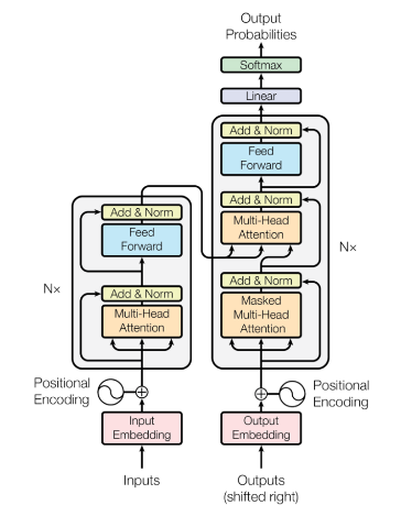
Position Embeddings: sines and cosines

$$
PE_{\text{(pos, 2i)}} = \sin(\text{pos}/10000^{2i/d_\text{model}})
$$

$$
PE_{\text{(pos, 2i+1)}} = \cos(\text{pos}/10000^{2i/d_\text{model}})
$$

Feed Forward Activation: ReLU

$$
FFN(x) = \max(0, xW_1+b_1)W_2 + b_2
$$

Norm: LayerNorm, applied after the residual stream is added back (Post-Norm)

Normalization

Pre-vs-post Norm

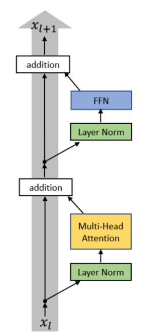
Originally, LayerNorm was applied after the “sublayer output + residual connection”:

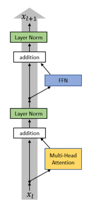
- Here, input $x_l$ is first sent to the attention module. Then, output of the attention is summed with the residual stream.
- Then, the normalized summation is sent to the feedforward layer, which is again summed with the residual stream.
- Finally, a LayerNorm is applied again before it is sent to the next layer.

$$
\begin{align}
x_{l, i}^{post, 1} &= MultiHeadAttn(x_{l, i}^{post}, [x_{l, 1}^{post}, \dots, x_{l, n}^{post}]) & \text{Sublayer Output (Attention)}\\
x_{l, i}^{post, 2} &= x_{l, i}^{post} + x_{l, i}^{post, 1} & \text{Residual Connection}\\
x_{l, i}^{post, 3} &= LayerNorm(x_{l, i}^{post, 2}) & \text{Norm after sublayer output + residual connection, i.e. PostNorm} \\
x_{l, i}^{post, 4} &= ReLU(x_{l, i}^{post, 3} W^{1,l}+b^{1, l})W^{2, l} + b^{2, l} & \text{Sublayer Output (Feedforward)}\\
x_{l, i}^{post, 5} &= x_{l, i}^{post, 3} + x_{l, i}^{post, 4} & \text{Residual Connection}\\
x_{l, i}^{post, 6} &= LayerNorm(x_{l, i}^{post, 5}) & \text{PostNorm} \\
\end{align}
$$

- Now, almost all modern LMs use pre-norm, which simply changes the order of the sandwich:

$$
\begin{align}
x_{l, i}^{pre, 1} &= LayerNorm(x_{l, i}^{pre}) & \text{Norm before sublayer output + residual connection, i.e. PreNorm} \\
x_{l, i}^{pre, 2} &= MultiHeadAttn(x_{l, i}^{pre, 1}, [x_{l, 1}^{pre, 1}, \dots, x_{l, n}^{pre, 1}]) & \text{Sublayer Output (Attention)}\\
x_{l, i}^{pre, 3} &= x_{l, i}^{pre} + x_{l, i}^{pre, 2} & \text{Residual Connection}\\
x_{l, i}^{pre, 4} &= LayerNorm(x_{l, i}^{pre, 3}) & \text{PreNorm} \\
x_{l, i}^{pre, 5} &= ReLU(x_{l, i}^{pre, 4} W^{1,l}+b^{1, l})W^{2, l} + b^{2, l} & \text{Sublayer Output (Feedforward)}\\
x_{l, i}^{pre, 6} &= x_{l, i}^{pre, 3} + x_{l, i}^{pre, 5} & \text{Residual Connection}\\
\end{align}
$$

In this case, LayerNorm is also applied before it is sent to the output head:

$$
x_{Final, i}^{pre} = LayerNorm(x_{L+1, i}^{pre})
$$

- Reason for the switch:
  - Training stability
  - Removes the need for the warmup iterations
  - Lets you use larger learning rates

Other approaches:
- Grok and Gemma-2 does double norm:

$$
\begin{align}
x_{l, i}^{double, 1} &= LayerNorm(x_{l, i}^{double})\\
x_{l, i}^{double, 2} &= MultiHeadAttn(x_{l, i}^{double, 1}, [x_{l, 1}^{double, 1}, \dots, x_{l, n}^{double, 1}])\\
x_{l, i}^{double, 3} &= LayerNorm(x_{l_i}^{double, 2})\\
x_{l, i}^{double, 4} &= x_{l, i}^{double} + x_{l, i}^{double, 3}\\
x_{l, i}^{double, 5} &= LayerNorm(x_{l, i}^{double, 4}) \\
x_{l, i}^{double, 6} &= ReLU(x_{l, i}^{double, 5} W^{1,l}+b^{1, l})W^{2, l} + b^{2, l}\\
x_{l, i}^{double, 7} &= LayerNorm(x_{l, i}^{double, 6})\\
x_{l, i}^{double, 8} &= x_{l, i}^{double, 4} + x_{l, i}^{double, 7}\\
\end{align}
$$

- Olmo 2 does only non-residual post norm:

$$
\begin{align}
x_{l, i}^{olmo, 1} &= MultiHeadAttn(x_{l, i}^{olmo}, [x_{l, 1}^{olmo}, \dots, x_{l, n}^{olmo}])\\
x_{l, i}^{olmo, 2} &= LayerNorm(x_{l_i}^{olmo, 1})\\
x_{l, i}^{olmo, 3} &= x_{l, i}^{olmo} + x_{l, i}^{olmo, 2}\\
x_{l, i}^{olmo, 4} &= ReLU(x_{l, i}^{olmo, 3} W^{1,l}+b^{1, l})W^{2, l} + b^{2, l}\\
x_{l, i}^{olmo, 5} &= LayerNorm(x_{l, i}^{olmo, 4}) \\
x_{l, i}^{olmo, 6} &= x_{l, i}^{olmo, 3} + x_{l, i}^{olmo, 5} \\
\end{align}
$$

LayerNorm vs. RMSNorm

Original transformer (along with GPT 3/2/1, OPT, GPT-J, BLOOM) uses LayerNorm:

$$
y = \frac{x – \mathbb{E}[x]}{\sqrt{Var[x] + \epsilon}} * \gamma + \beta
$$

Most new models (e.g. LLaMA-family, PaLM, Chinchilla, T5) use RMSNorm:

$$
y = \frac{x}{\sqrt{\dfrac{||x||^2_2}{n} + \epsilon}} * \gamma
$$

- Removes bias term $\to$ Fewer parameters to store
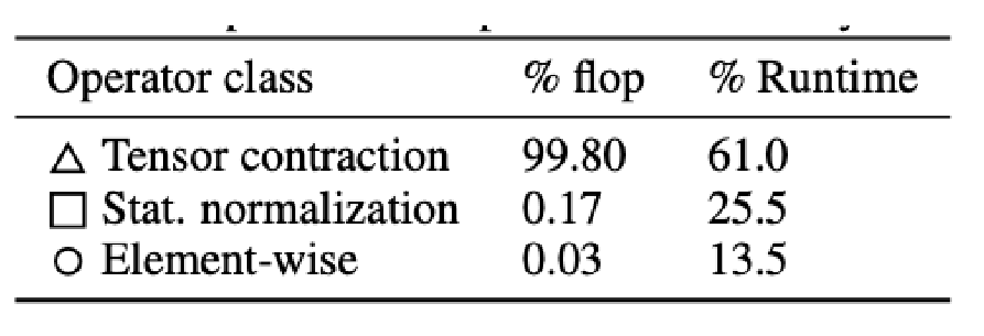
- Does not calculate and subtract the mean $\to$ Fewer operations
Even though most of the FLOPs happen during the matrix multiplication, bias term and normalization operation can still increase the runtime due to required data movement operations:

Bias Terms

Original transformer and earlier models used bias terms:

$$
FFN(x) = \max(0, xW_1 + b_1)W_2 + b_2
$$

Most newer (but non-gated) implementations get rid of the bias term for performance gain and to store less parameters:

$$
FFN(x) = \sigma(xW_1)W_2
$$

Activations

Earlier, ReLU and GeLU were the most commonly used.
- ReLU:

$$
FF(x) = \max(0, xW_1)W_2
$$

GeLU:

$$
\begin{align}
FF(x) &= GELU(xW_1)W_2 &\\
GELU(x) &:= x \Phi(x) & \Phi(.) \text{ is the Gaussian CDF}
\end{align}
$$

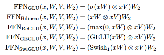
New trend is to use gated activations. Idea is:
- Project the input into two different vectors, let’s say $g$ and $p$.
- $g$ is sent through a nonlinear function, turns into “gate weights”.
- $g$ and $p$ is then element-wise multiplied.
So, instead of two weight matrices per FFN like in the original transformer, now we have 3.
- That is why gated models use smaller internal dimensions by about 2/3, so the number of parameters for FFN is roughly the same.
Examples:

Serial and Parallel Layers

Standard transformer block applies first attention, and then the feedforward layer.
Serial implementation is still the standard practice, but there are alternative approaches for speed gain.

$$
\begin{align}
y &= x + \underbrace{MLP(\text{LayerNorm}(x + \text{Attention}(\text{LayerNorm}(x))))}_{\text{Working on the normalized residual stream + attention layer outputs}} & \text{Serial Transformer Block} \\
y &= x + \underbrace{MLP(\text{LayerNorm}(x))}_{\text{Working only on normalized input}} + \text{Attention}(\text{LayerNorm}(x)) & \text{Parallel Transformer Block}
\end{align}
$$

Position Embeddings

Sine – Cosine Embeddings
- Use sine and cosine to keep track of the token positions.
- Embedding for a token $x$ at position $pos$:

$$
\begin{align}
Embed(x, pos) &= v_x + PE_\text{pos}\\
PE_{(pos, 2i)} &= \sin(pos/10000^{2i/d_\text{model}}) \\
PE_{(pos, 2i+1)} &= \cos(pos/10000^{2i/d_\text{model}}) \\
\end{align}
$$

- Idea is to create an embedding matrix $PE$, where each row corresponds to a position vector. In the beginning dimensions of the vector, you have higher frequency functions, and in the ending dimensions you have lower frequency functions.
- So, dimensions near the end are better to understand the ballpark position, and the earlier dimensions are to precisely determine the position.
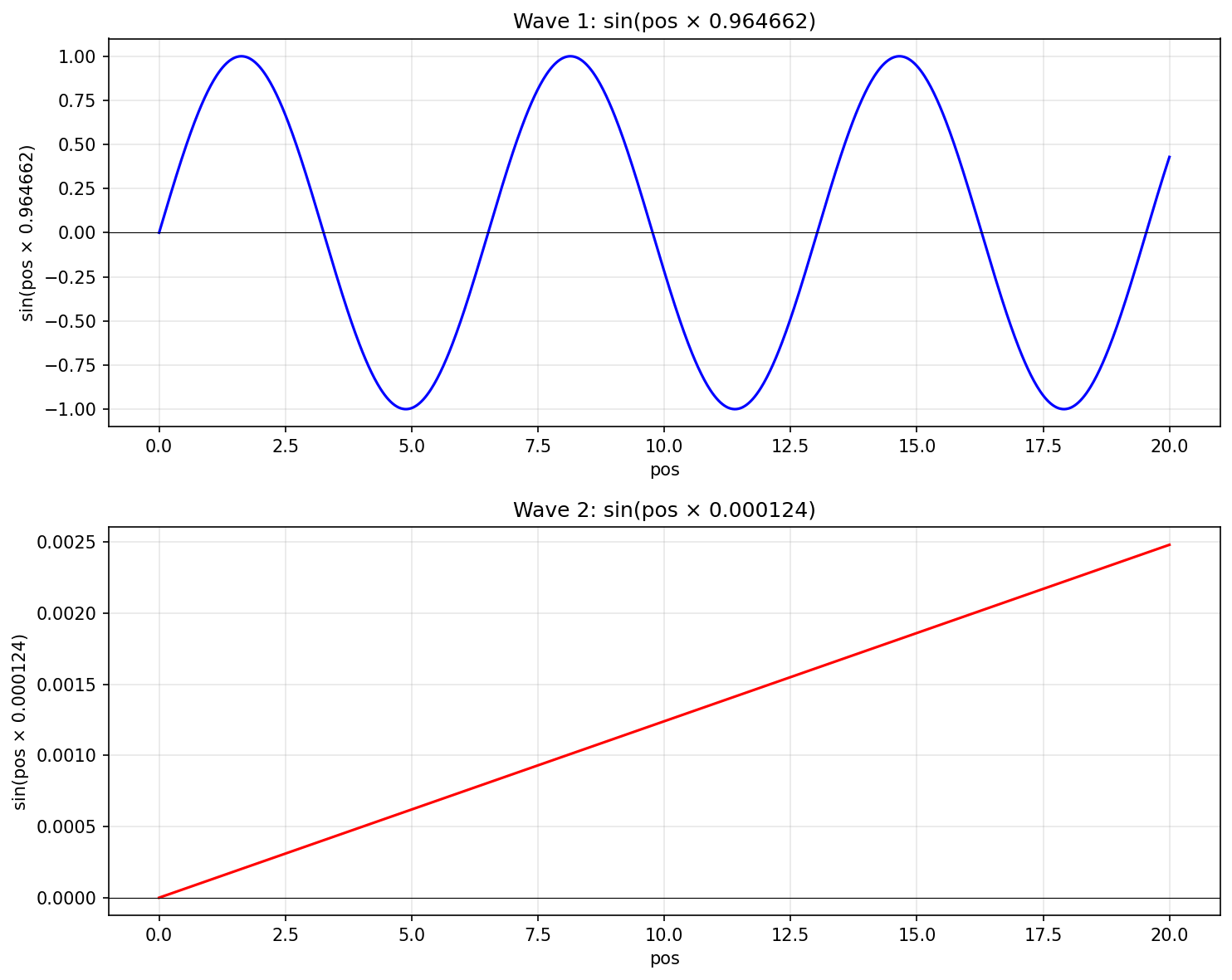
  - Assume $d_\text{model} = 1024$
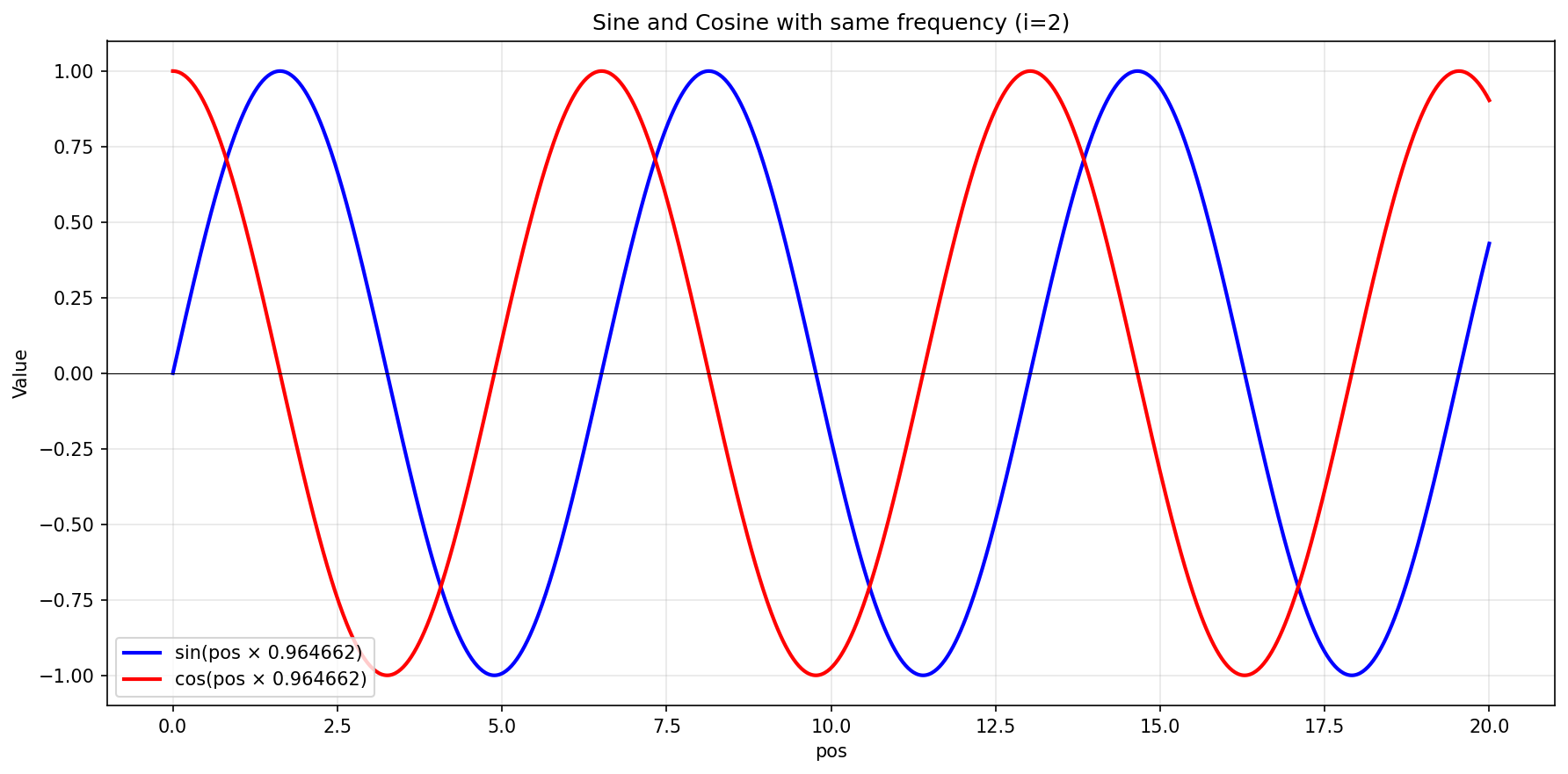
  - This means we have $512$ sine waves, and $512$ cosine waves, each with different frequency. Let’s focus on the sine waves at $i=2$, and $i=500$.

$$
\begin{align}
\sin(pos \times \frac{1}{10000^{4/1024}}) &\approx \sin(pos\times 0.964662) & (i=2)\\
\sin(pos \times \frac{1}{10000^{1000/1024}}) &\approx \sin(pos\times 0.000124) & (i=500)
\end{align}
$$

- - Now, notice that the sine wave with $i=500$ changes much slower compared to the wave with $i=2$, because it has lower angular frequency, i.e $0.000124 < 0.964662$. That is why, that dimension changes much slower ($\sim 7800$ times slower).
  - Here, you can see how they change for the first $20$ positions:

- - First function will complete its cycle around $6.51$ positions and start repeating, while the second function completes its cycle in around $50645$ positions:

$$
\begin{align}
\omega_{i=2} = \frac{2\pi}{T} = 0.964662 \implies T \approx \frac{2\times3.14}{0.964662} \approx 6.51\\
\omega_{i=500} = \frac{2\pi}{T} = 0.000124 \implies T \approx \frac{2\times3.14}{0.000124} \approx 50645
\end{align}
$$

- - So, the high frequency function can only determine position up to $6.51$ units, and then has to start repeating.
  - Lower frequency function completes its cycle much later, so it can determine positions up to $50645$ units. But because it changes so slowly, it can not discriminate between e.g. $pos=2$ and $pos=3$ (See how close they are in the plot above).
  - That was the rationale behind using trigonometric functions.
    - And also they thought model could learn to exploit the trigonometric identities to do “relative positioning too”, but this doesn’t seem to be the case.

But idea was:

$$
\begin{align}
& \sin(pos+k) = \sin(pos)\cos(k) + \cos(pos)\sin(k)\\
& \cos(pos+k) = \cos(pos)\cos(k) – \sin(pos)\sin(k)\\ \\
\implies &
\begin{bmatrix}
\sin(pos+k)\\
\cos(pos+k)
\end{bmatrix} =
\underbrace{ \begin{bmatrix}
\cos(k) & \sin(k) \\
-\sin(k) & \cos(k)
\end{bmatrix}}_{A}\times
\underbrace{\begin{bmatrix}
\sin(pos)\\
\cos(pos)
\end{bmatrix}}_{\text{PE}}
\end{align}
$$

- - And this is just a linear operation, a matrix multiplication between some weights $A$ and the positional embeddings matrix PE.
- Furthermore, instead of using only sine, they also used cosine at the same frequency. This helps to differentiate between e.g. position 3 and 6, where for $i=2$, sines will have almost exactly the same value but cosines will be different:

Absolute Embeddings
- Used in GPT-1, 2, 3 and OPT
- Instead of using fixed positional embeddings like the trigonometric ones before, turn it into a trainable layer

$$
Embed(x, pos) = v_x + u_\text{pos}
$$

Relative Embeddings
- Used in T5, Gopher, Chinchilla
- Instead of adding a learned or fixed position embedding to the token, use a learned embedding based on the offset between the “key” and “query” in the attention layers.
- A fixed number of embeddings are learned, corresponding to a range of possible key-query offsets.
- Start with the classic scaled dot-product attention between $x_i$ and $x_j$:

$$
e_{ij} = \frac{\overbrace{(x_iW^Q)}^{Query}\overbrace{(x_jW^K)^T}^{Key}}{\underbrace{\sqrt{d_z}}_{Normalization}}
$$

Define two learnable vectors for the relationship between $x_i$ and $x_j$, one on the value level and one on the key level: $a_{ij}^V, a_{ij}^K \in \mathbb{R}^{d_a}$.
- These relationship vectors can be shared between different attention layers.
Then, you can simply add these relative vectors to where you originally use key and value vectors.
To calculate the context vectors:

$$
\underbrace{z_i}_{\text{Context vector for token at position i}} = \sum_{j=1}^n \alpha_{ij}\underbrace{(\underbrace{x_jW^V}_{\text{Value Vector for $x_j$}} + \underbrace{a_{ij}^V}_{\text{Value vector for positions [i] and [j]}})}_{\text{Modified value vector}}
$$

To calculate the attention scores:

$$
e_{ij} = \frac{\overbrace{x_i W^Q}^{\text{Query vector for $x_i$}}\overbrace{(\overbrace{x_jW^K}^{\text{Key vector for $x_j$}} + \overbrace{a_{ij}^K}^{\text{Key vector for positions [i] and [j]}})^T}^{\text{Modified key vector for $x_j$}}}{\sqrt{d_z}}
$$

Because it is impractical to model all possible differences, and arguably not needed, maximum distance $|i – j|$ is clipped at some value $k$ and then gets repeated. This means it will be possible to model $2k+1$ unique distances. ($k$ in both directions):

$$
\begin{align}
a_{ij}^K &= w_\text{clip(j-i, k)}^K \\
a_{ij}^V &= w_\text{clip(j-i, k)}^V \\
\text{clip}(x, k) &= \max(-k, \min(k, x))
\end{align}
$$

- Efficient implementation:
  - While theoretically it is nicer to think in terms of “modifying” the key and value vectors, efficient implementation actually does not modify the key matrices but adds another matrix multiplication, which is mathematically equivalent:

$$
e_{ij} = \frac{x_iW^Q(x_jW^K)^T+x_iW^Q(a_{ij}^K)^T}{\sqrt{d_z}}
$$

ALiBi (Attention with Linear Biases)
- Similar to the idea of relative embeddings, can be considered a special case.
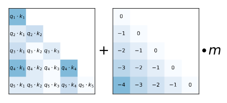
- We are modifying the attention score calculation, using non-learnable bias terms:

$$
\begin{align}
e_{ij} = \frac{x_iW^Q(x_jW^K)^T}{\sqrt{d_z}} + m\cdot(j-i)
\end{align}
$$

Here, $m$ is a predetermined scalar changing the slope for the different heads, going up to $\frac{1}{2^8}$. For 8 attention heads, they have $\frac{1}{2^1}, \frac{1}{2^2}, \dots, \frac{1}{2^8}$ and for 16 attention heads, it is $\frac{1}{2^{0.5}}, \frac{1}{2^{1}}, \dots, \frac{1}{2^{7.5}}, \frac{1}{2^{8}}$. (So, basically start from $2^{\frac{-8}{n}}$ and go up to $2^{-8}$) .
Idea is, for each token, causal attention calculation is done only based on the per-token representation so far, and then bias term provides the position information by punishing the distant terms, i.e. a closer token will have $-m + \text{score}$ and if the distance in between is 10 tokens, it will be $-10m + \text{score}$. And each head “punishes” the distance separately, based on their pre-determined slope:

As the distance gets longer, the $m\times\text{distance}$ term will start to dominate the actual score, so applying softmax to them will create outputs near $0$, i.e. because you are pushing the far-away tokens to be more negative/smaller, and closer tokens only slightly, softmax will favor the closer tokens.
Expectation is, that this is going to learn to generalize to unseen context lengths, thanks to its recency bias. However, this could be problematic when you need long-term dependencies.
RoPE (Rotary Positional Embeddings)
- Think of the modeling of the relative distance in the attention layers:

$$
\begin{align}
\langle f_q(x_m, m), f_k(x_n, n) \rangle &= g(x_m, x_n, m-n)
\end{align}
$$

where $x_m$ is the query token at position $m$, and $x_n$ is the key token at position $n$. The goal is to end-up with a function $g$, that should calculate an attention score based on three inputs:

- $x_m$: Embedding for $x_m$
- $x_n$: Embedding for $x_n$
- $m-n$: Distance between the positions of $x_m$ and $x_n$
First, remember the rotation matrices in 2D, and how they are defined using $\sin$ and $\cos$ functions of the same frequency:

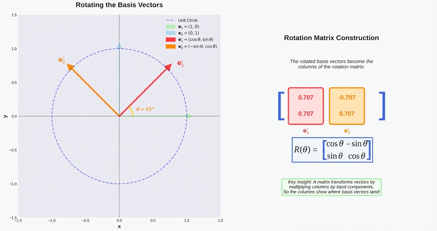
Original transformer used pairs of sines and cosines as well, but for absolute encoding. Now, idea is to use the same sines and cosines, but instead of adding them to the token embeddings, we will rotate the key and query vectors at attention layers. Rotation matrix is defined similarly:

$$
\begin{align}
R_{\Theta, m}^d &= \begin{pmatrix} \cos m\theta_1 & -\sin m \theta_1 & 0 & 0 & \cdots & 0 & 0 \\ \sin m\theta_1 & \cos m \theta_1 & 0 & 0 & \cdots & 0 & 0 \\ 0 & 0 & \cos m\theta_2 & -\sin m \theta_2 & \cdots & 0 & 0 \\ 0 & 0 & \sin m\theta_2 & \cos m \theta_2 & \cdots & 0 & 0 \\ \vdots & \vdots & \vdots & \vdots & \ddots & \vdots & \vdots \\ 0 & 0 & 0 & 0 & \cdots & \cos m \theta_{d/2} & -\sin m\theta_{d/2} \\ 0 & 0 & 0 & 0 & \cdots & \sin m \theta_{d/2} & \cos m \theta_{d/2} \\ \end{pmatrix}\\[1em] \\
&= \begin{pmatrix} \mathbf{R}(\theta_1) & \mathbf{0} & \cdots & \mathbf{0} \\ \mathbf{0} & \mathbf{R}(\theta_2) & \cdots & \mathbf{0} \\ \vdots & \vdots & \ddots & \vdots \\ \mathbf{0} & \mathbf{0} & \cdots & \mathbf{R}(\theta_{d/2}) \end{pmatrix} \end{align} \\
$$

So, we have $d/2$ different rotation matrices, which are defined based on cosine and sine functions with different frequencies. Base frequency is the same one as they had in the original transformer:

$$
\Theta = \{ \theta_i = \frac{1}{10000^{2(i-1)/d}}, i \in [1, 2, \dots, d/2] \}
$$

Then, you have to rotate your query and key vectors, and every two dimension rotate in different frequencies (frequencies have been changed so their movement can be shown in the animation):

Then, you simply rotate both your query and key vectors when you are calculating the attention scores:

$$
\begin{align}
q’_m &= R^d_{\Theta,m} W_q x_m & \text{(Rotated query vector for token at position m)}\\
k’_n &= R^d_{\Theta, n} W_k x_n & \text{(Rotated key vector for token at position n)}\\
e_{ij} &= \dfrac{(R^d_{\Theta,m} W_q x_m)^T (R^d_{\Theta, n} W_k x_n)}{\sqrt{d}} = \dfrac{x^T_m W_q \overbrace{R_{\Theta, (n-m)}^d}^{\text{Relative rotation}} W_k x_n}{\sqrt{d}}
\end{align}
$$

So, rotating the query vector and value vector by their absolute positions corresponds to using a rotation matrix based on relative positions, as:

$$
\begin{align}
R(n\theta) \cdot R(-m\theta) &=
\begin{bmatrix}
\cos n\theta & -\sin n\theta \\ \sin n\theta & \cos n\theta \end{bmatrix} \begin{bmatrix} \cos(-m\theta) & -\sin(-m\theta) \\ \sin(-m\theta) & \cos(-m\theta) \end{bmatrix}\\[1em] &= \begin{bmatrix} \cos n\theta & -\sin n\theta \\ \sin n\theta & \cos n\theta \end{bmatrix} \begin{bmatrix} \cos m\theta & \sin m\theta \\ -\sin m\theta & \cos m\theta \end{bmatrix}\\[1em] &= \begin{bmatrix} \cos n\theta \cos m\theta + \sin n\theta \sin m\theta & \cos n\theta \sin m\theta – \sin n\theta \cos m\theta \\ \sin n\theta \cos m\theta – \cos n\theta \sin m\theta & \sin n\theta \sin m\theta + \cos n\theta \cos m\theta \end{bmatrix}\\[1em] &= \begin{bmatrix} \cos(n-m)\theta & -\sin(n-m)\theta \\ \sin(n-m)\theta & \cos(n-m)\theta \end{bmatrix}\\[1em] &= R((n-m)\theta)
\end{align}
$$

Efficient Implementation
- Because the rotation matrix is sparse, it is possible to do the multiplication computationally more efficient with:

$$
R^d_{\Theta,m} \mathbf{x} =
\begin{pmatrix}
x_1 \\
x_2 \\
x_3 \\
x_4 \\
\vdots \\
x_{d-1} \\
x_d
\end{pmatrix}
\otimes
\begin{pmatrix}
\cos m\theta_1 \\
\cos m\theta_1 \\
\cos m\theta_2 \\
\cos m\theta_2 \\
\vdots \\
\cos m\theta_{d/2} \\
\cos m\theta_{d/2}
\end{pmatrix}
+
\begin{pmatrix}
-x_2 \\
x_1 \\
-x_4 \\
x_3 \\
\vdots \\
-x_d \\
x_{d-1}
\end{pmatrix}
\otimes
\begin{pmatrix}
\sin m\theta_1 \\
\sin m\theta_1 \\
\sin m\theta_2 \\
\sin m\theta_2 \\
\vdots \\
\sin m\theta_{d/2} \\
\sin m\theta_{d/2}
\end{pmatrix}
$$

Hyperparameters

Field seems to converge on some hyperparameters:

Feedforward – model dimension ratio
- Usually is scaled up to 4 times of the model dimension and scaled back down.

$$
d_{ff} = 4 d_\text{model}
$$

- GLU variants: Because researchers wanted to keep the parameter count similar, they tend to scale down the hidden size of the feedforward layer:

$$
d_{ff} \approx \frac{8}{3}d_\text{model}
$$

Number of heads and head dimension
- Usually, number of heads and dimension of the heads is chosen in a way, such that their multiplication is equal to the model dimension:

$$
d_\text{model} = n_\text{heads} \times d_\text{head}
$$

Depth (number of layers) vs. width (model dimension) debate
- Earlier, there were very deep models (BLOOM, T5 v1.1) with $d_\text{model}/n_\text{layer} > 170$, and very wide models (T5, GPT-2) with $d_\text{model}/n_\text{layer} < 50$, but newer models usually have the following aspect ratio:

$$
100 < \dfrac{d_\text{model}}{n_\text{layer}} < 160 $$

- The choice of depth and width is also affected by your networking constraints and the type of parallelisms you can do. e.g. Tensor parallel that lets you train wider networks need fast network, while pipeline parallel where you can shard the model per layer can get away with a slower network.
- But empirical research (OpenAI Scaling paper) shows the sweet spot is around 70 – 150
Vocabulary sizes
- Monolingual models usually have around 30,000 – 50,000 token vocabulary size
- Multilingual and newer models have between 64,000 – 255,000 token vocabulary size
Training regularization
- Initially, a lot of models were using dropout
- Nowadays, it seems like most don’t use dropout anymore, but switched to using weight decay
- However, weight decay is not used for regularization, as it looks like it has no effect on overfitting (i.e. ratio of training loss to validation loss), but rather has an interesting relationship to dynamic learning rates like cosine LR decay, and ends up facilitating faster training and higher accuracy. Furthermore, weight decay stabilizes training with bfloat16.
- More on this at D'Angelo, Francesco, et al. "Why do we need weight decay in modern deep learning?." <em>Advances in Neural Information Processing Systems</em> 37 (2024): 23191-23223.

Stability Tricks

Softmaxes -> The problem child
- Used in the final layer and also attention layers
- Solution for the Final Layer: Z-loss (from 2014 – Devlin et. al., for decoding speed, later used for stability in 2022 by PaLM)
  - Z-loss refers to the normalization factor in softmax. Softmax if defined as:

$$
P(x)_i = \sigma(x)_i = \frac{\exp(x_i)}{\underbrace{\sum_{j=1}^d \exp(x_j)}_{\text{Z($x$), i.e. Softmax Normalizer}}}
$$

- - It turns out, by encouraging the normalizer to be close to $1$, we can get more stable training runs. As you can write the log likelihood as log softmax, loss calculation on softmax can be written as:

$$
\begin{align}
L(x) &= \log\left(\frac{\exp(x_i)}{Z(x)}\right) \\
&= \log(\exp(x_i)) – \log(Z(x))
\end{align}
$$

, assuming logit $i$ represents the correct logit.

- - Then, to encourage the $Z(x)$ to be $1$, you can simply push the $\log(Z(x))$ towards 0, with a coefficient of $\alpha$ where $\alpha$ determines the amount of “encouragement”:

$$
\begin{align}
L(x) &= \left[ \log(P(x)_i) – \alpha (\log(Z(x)) – 0)^2 \right] \\
&= [\log(P(x)_i) – \alpha \log^2 (Z(x)) ] \\
&= [\underbrace{\log(\exp(x_i)) – \log(Z(x))}_{\text{Standard Softmax Loss}} – \underbrace{\alpha\log^2(Z(x))}_{\text{Z-loss}}]
\end{align}
$$

- - In PaLM, $\alpha = 10^{-4}$.
  - So, the idea is to add additional MSE loss on $\log(Z(x))$. In theory, you can apply this to all softmax layers but in practice, everyone just applies it to the last layer.
- For the attention softmaxes, another trick is used, namely QK Norm.
  - Idea is simple. Before you calculate the attention with dot product of $q$ and $k$, apply LayerNorm / RMSNorm on them.

Attention Heads

Cost of the Multi-Head Attention

There are various alternatives to multi-head attention, devised in order to make best use of the GPU time. To understand why, let’s calculate the cost of attention in each head.

Every head computes three projections first:

$XW^Q \to$ Projects inputs to the query vectors
$XW^K \to$ Projects inputs to the key vectors
$XW^V \to$ Projects inputs to the value vectors

(We will drop the batch size from calculations for simplicity)

Assuming $X \in \mathbb{R}^{n\times d}$ and $W^Q, W^K, W^V \in \mathbb{R}^{d \times d_a}$:

Computational cost of projections: $O(ndd_a)$.
Memory cost: $O(nd + dd_a)$
- You could also include the output activations for memory, i.e. $O(nd + dd_a + nd_a)$ but since $d > d_a$ almost always, I drop it)

Then, the resulting matrices $Q, K \in \mathbb{R}^{n\times d_a}$ are multiplied to get $QK^T$:

Computational cost: $O(n^2d_a)$
Memory cost: $O(nd_a + n^2)$

Now, the resulting matrix $QK^T \in \mathbb{R}^{n\times n}$ will have softmax applied to it.

Computational cost: $O(n^2)$
Memory cost: $O(n^2)$

Now that we have the attention scores, we want to create the context vectors by multiplying the attention scores and the value vectors. As we are multiplying two matrices with sizes $(n\times n) \times (n \times d_a)$:

Computational cost: $O(n^2d_a)$
Memory cost: $O(n^2 + nd_a)$

Now, this is the key insight here. As we are doing this for every head, all of the calculations get multiplied with $h$ (except the memory cost of the input matrix, it doesn’t get read from the memory for each head)! So, so far we have

Computational cost: $O(hndd_a + hn^2d_a + hn^2 + hn^2d_a) \to O(hndd_a + hn^2d_a)$
- Note: This can further simplify depending on the relationship between $n$ and $d$, but with the modern models we are not sure what the sequence length is going to be compared to the dimension of the model
Memory cost:

$$
\begin{align}
O(&\underbrace{nd}_{\text{Input to attention for projections}} + \underbrace{hdd_a}_{\text{Output of the projections}} + \underbrace{hnd_a}_{\text{Input for attention score}} + \underbrace{hn^2}_{\text{Output for attention score}} + \\
& \underbrace{hn^2}_{\text{Softmax Activations}} + \underbrace{hn^2}_{\text{Input to context vector calculation}} + \underbrace{hnd_a}_{\text{Output of the context vector calculation}}) \\
& \to O(\underbrace{nd}_{\text{Input to attention for projections}} + \underbrace{hn^2}_{\text{Attention score outputs + softmax activations + context vector calculation input}})
\end{align}
$$

Then, after head outputs are combined (this is a memory operation, so you can maybe incur an $O(nd)$ memory cost again but doesn’t change the calculations), you have the final projection $CP$, with $C \in \mathbb{R}^{n\times d}, P \in \mathbb{R}^{d\times d}$ context matrix and projection matrix, respectively. This final operation has:

Computational cost: $O(nd^2)$
Memory cost: $O(nd + d^2)$

Combining everything together,

Total computational cost: $O(hndd_a + hn^2d_a + nd^2)$
Total memory cost: $O(nd + hn^2 + d^2)$

Now, we can do some assumptions based on the general conventions. Usually, $d = h\times d_a$. Then:

Computational cost: $O(nd^2 + n^2d)$
Memory cost: $O(nd + hn^2 + d^2)$

So, this computational cost and memory cost showed us something. With the current conventions, number of heads has negligible effect on the computational cost but memory cost is highly dependent on the number of heads. Ideally, we want to improve arithmetic intensity, that is the ratio of computational cost to memory cost. As we do not want to have smaller hidden dimensions or shorter sequences, we tend to play around with the number of heads to improve the arithmetic intensity.

Batching Multi-Head Attention

For simplicity, we dropped the batch from the calculations. Lets add it back:
- Computational Cost: $O(bnd^2 + bn^2d)$
- Memory Cost: $O(bnd + bhn^2 + d^2)$ (Projection matrix is independent of the batch size, so it does not get multiplied by $b$)
- Arithmetic Intensity: $O\left(\frac{bnd^2 + bn^2d}{bnd + bhn^2 + d^2}\right)$
During training, this can be accepted, because by batching you can parallelize all the operations and still utilize the GPUs fully.
However, during the inference time, each attention calculation has to wait for the memory movement. So, you get into Generate -> IO Wait -> Generate -> IO Wait -> Generate … workflow. This under-utilizes the GPU (if not enough parallel requests) and causes slow responses (due to waiting for memory movement).

Multi-Query Attention (MQA)

Proposed Solution: Have queries per head, but share the $W^K$ and $W^V$
What does it achieve:
- In MHA, for each head data movement per key and value matrices is $O(hnd_a) = O(nd)$.
- By having only one Key and Value matrix, we decrease the memory movements by a factor of $h$ -> $O(nd_a)$
- Even though this does not change the full complexity analysis, it provides significant speed-ups in reality because you significantly reduce the data movement from KV cache (this is primarily an inference optimization).

Grouped-Query Attention (GQA)

Proposed Solution: MQA can decrease performance, so have shared key and value matrices, e.g. first key and value matrices will be used by the first 3 heads, the second will be used by the heads 3-6 and so on.

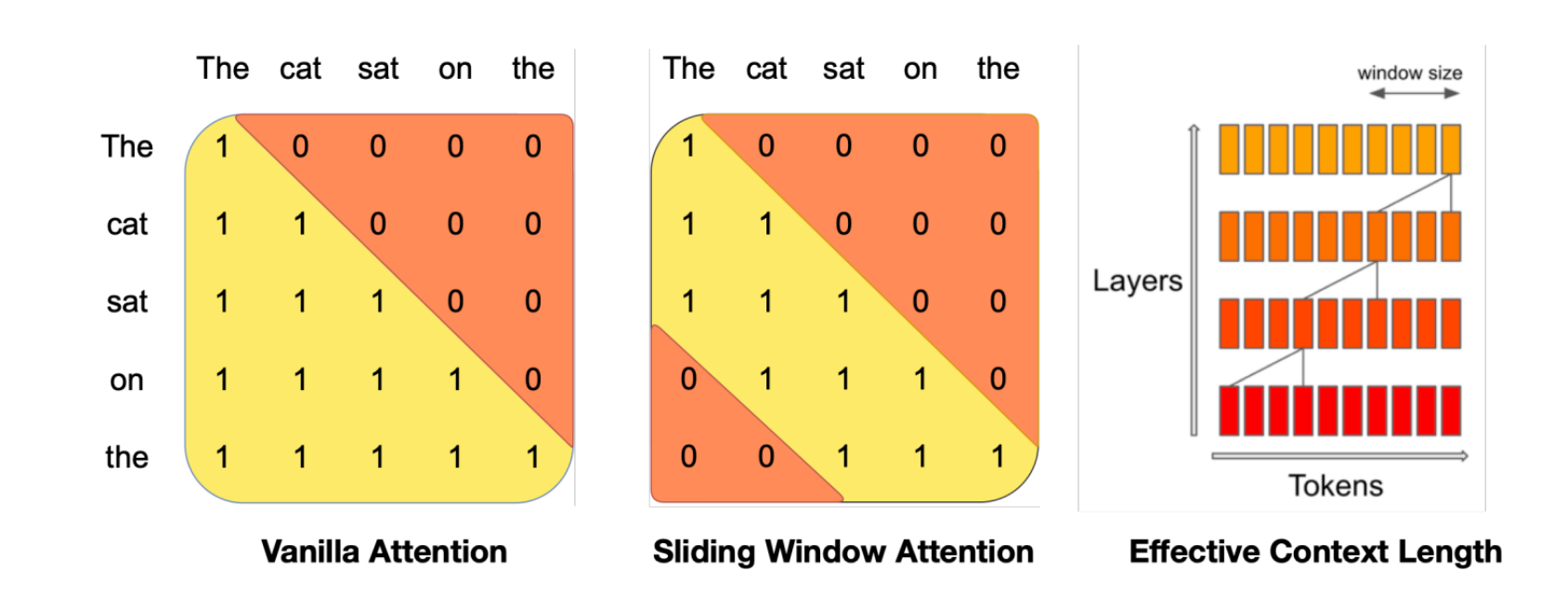
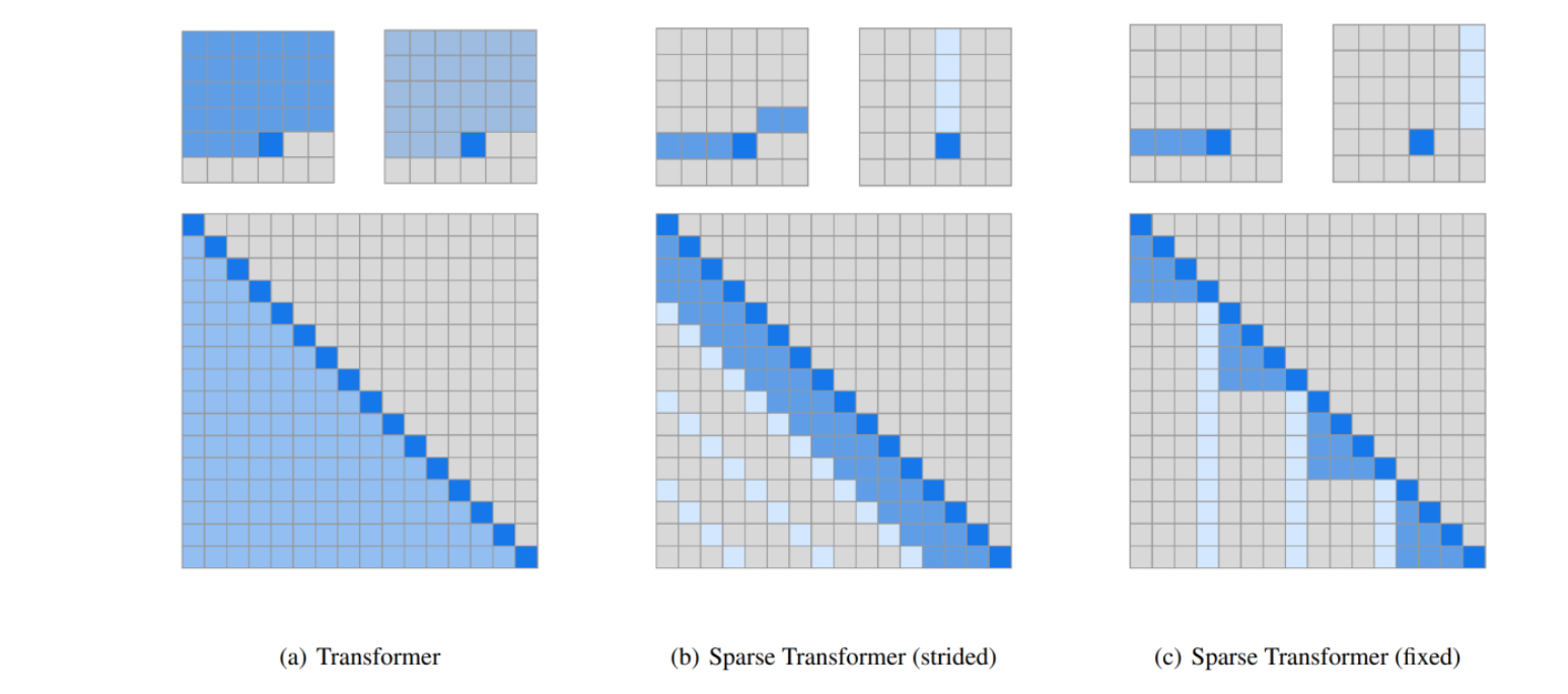
Sparse and Sliding Window Attentions

Basically, consider only the closest tokens:
Sliding Window attention:
Sparse Transformers:

Combining Long- and Short-Range Information

E.g. in Cohere Command A, every 4th layer is a full attention layer with no positional embeddings (NoPE).
Other attention layers are Sliding Window + Grouped Query Attention with RoPE.

Resources:

Language Modeling from Scratch Lecture Notes – Percy Liang, Tatsunori Hashimoto, Stanford University https://stanford-cs336.github.io/spring2025/

Shazeer, Noam. “Glu variants improve transformer.” arXiv preprint arXiv:2002.05202 (2020).

Vaswani, Ashish, et al. “Attention is all you need.” Advances in neural information processing systems 30 (2017).

Shaw, Peter, Jakob Uszkoreit, and Ashish Vaswani. “Self-Attention with Relative Position Representations.” Proceedings of NAACL-HLT. 2018.

Xiong, Ruibin, et al. “On layer normalization in the transformer architecture.” International conference on machine learning. PMLR, 2020.

Ivanov, Andrei, et al. “Data movement is all you need: A case study on optimizing transformers.” Proceedings of Machine Learning and Systems 3 (2021): 711-732.

Press, Ofir, Noah A. Smith, and Mike Lewis. “Train short, test long: Attention with linear biases enables input length extrapolation.” arXiv preprint arXiv:2108.12409 (2021).

Su, Jianlin, et al. “Roformer: Enhanced transformer with rotary position embedding.” Neurocomputing 568 (2024): 127063.

Devlin, Jacob, et al. “Fast and robust neural network joint models for statistical machine translation.” proceedings of the 52nd annual meeting of the Association for Computational Linguistics (Volume 1: Long Papers). 2014.

Chowdhery, Aakanksha, et al. “Palm: Scaling language modeling with pathways.” Journal of Machine Learning Research 24.240 (2023): 1-113.

Andriushchenko, Maksym, et al. “Why do we need weight decay in modern deep learning?.” (2023).

“Multi-Query Attention is All You Need.” Fireworks AI, https://web.archive.org/web/20251224025619/https://fireworks.ai/blog/multi-query-attention-is-all-you-need

Ainslie, Joshua, et al. “Gqa: Training generalized multi-query transformer models from multi-head checkpoints.” arXiv preprint arXiv:2305.13245 (2023).

Child, Rewon. “Generating long sequences with sparse transformers.” arXiv preprint arXiv:1904.10509 (2019).

Jiang, Albert Q., et al. “Mistral 7B.” arXiv, 10 Oct. 2023, doi:10.48550/arXiv.2310.06825.

Other figures are mostly created with the help of Claude Sonnet 4.5.

December 28, 2025December 28, 2025

Memory and Computation Cost of Large Language Models

I have recently started following/auditing Stanford’s CS336 course, and while going through the second lecture I took some notes which I think can be also valuable for others.. This lecture focuses on analysing the computation and memory cost of LLMs, with explanations. To understand them better, you also need to understand the computation graphs a little bit, which I added as an interlude from Andreas Geiger’s notes on the topic. Furthermore, I reiterated the OpenAI’s analysis on the memory and compute requirements, while trying to explain the reasoning.

Motivating Questions

How long would it take to train a 70B parameter model on 15T tokens on 1024 H100s?

Determine the total number of FLOPs you need
Get the FLOPs per second from the info sheet (H100: 1979e12 / 2)
Get model flops utilization -> A metric to measure efficiency of your training
Flops you can use per day: GPU Flops Capacity x Model Flops Utilization x Number of GPUs x Seconds in a Day
Then, the training will take “Needed number of FLOPs / FLOPS you can use per day” days.

What is the largest model that you can train on 8 H100s using AdamW (naively)?

Get the VRAM size of the GPU in bytes
Calculate the bytes you need per parameter (Depends on the precision you use and the optimizer)
Then, simply divide to find the biggest model you can train within the constraints

Note: This does not account for the cost of activations, which depend on the batch size and the sequence length.

Memory Accounting

Tensors are the basic building blocks for everything else.
Creating tensors without initializing values:

x = torch.empty(4, 8) # Create an empty 4, 8 matrix
nn.init.trunc_normal_(x, mean=0, std=1, a=-2, b=2) # Initialize the values in a specific way

Most tensors are stored as floating point numbers.

Reminder about Floating Point Representations

In real life, we use scientific notation to separate the interesting parts of the number and its order of magnitude.
For example, Avogadro number: $6.022 \times 10^{23}$.
- We say this number has 4 digits of precision, and this actually represents some range of possible measurements: $[ 6.022 \times 10^{23} – \varepsilon, 6.022 \times 10^{23} + \varepsilon ]$ where $\varepsilon \approx 0.001 \times 10^{23}$. (If $\varepsilon$ were to be larger, then it would be put into the digits of precision part, so we know our error must be smaller than $\varepsilon \times 10^{23}$)
In this case, $6.022$ is called the significand (or fraction) and $23$ is called the exponent.

float32 (=fp32=Single Precision)

32 bits, 1 for sign, 8 for exponent and 23 bits for the fraction.
It is the default.
In deep learning, unlike scientific computing, we do not use double precision (float64).
Memory is determined by the number of values, and types of those values.
- e.g. assume a (4, 8) matrix. Its memory cost is $4 \times 8 \times 32 = 1024$ bits, or $4\times8\times4 = 128$ bytes (8 bits = 1 byte, float32 = 4 bytes)
Example: One matrix in the feedforward layer of GPT-3:
- Embedding size: 12_288
- Matrix size: (12_288 * 4, 12_288)
- This means this matrix in single precision would cost 2306 MB, or 2.25 GB.
Maximum positive number you can represent: $\underbrace{(1 + \underbrace{8388607/8388608}_{\text{Fraction}})}_{\text{Mantissa}} \times 2^{127}$ (127 because half is used for the negative representation, and the upper and lower ends are reserved for special representations like 0, nan, infinity).
Notice how precise you can get, and range is given by the exponent bits.

float16 (=fp16=Half Precision)

16 bits, 1 sign, 5 exponent, 10 fraction.
Cuts the memory usage in half.
However, it is not great for small numbers, as e.g. 1e-8 would go to $0$
This can lead to underflows in gradient if used during training.
Maximum positive number you can represent: $\underbrace{(1 + \underbrace{1023/1024}_{\text{Fraction}})}_{\text{Mantissa}} \times 2^{15}$
Now, our mantissa is less precise, and our range is also smaller due to having less bits for exponents

bfloat16 (Brain Floating Point)

For deep learning, we care about the dynamic range more then we care about the fraction bit because we want to have more stable gradients.
Resolution is worse (fraction/significand can be represented with 7 bits), but it has the same dynamic range as the float32 while using half the space.
Developed by Google Brain
Maximum number you can represent: $\underbrace{(1 + \underbrace{127/128}_{\text{Fraction}})}_{\text{Mantissa}} \times 2^{127}$
Notice that our mantissa is more crude, but our range is as high as fp32 again.

fp8

Standardized in 2022
Only supported by H100 and later
There are two types:
- FP8 E4M3 (exponent 4, mantissa 3)
  - Cannot represent infinities, only NAN is defined
  - This increases the range of representable numbers
  - Maximum representable number: $(1 + 6/8) \times 2^8 = 448$
    - Because they decided not to make infinities representable, they increased dynamic range
    - Because NaN is defined as all bits set to 1, you cannot represent $1+7/8 \times 2^8$.
- FP8 E5M2 (exponent 5, mantissa 2)
  - Can represent infinities and NaN
  - Maximum representable number: $(1 + 3/4) \times 2^{15} = 57,344$
Forward activations and weights require more precision, so E4M3 datatypes are best used in the forward pass.
For the backward pass, range is more important for the gradients then the precision, so E5M2 can be utilized.

Practicality

To store parameters and optimizer states, you still need float32.
- Or training can go haywire.
- fp32 -> Safe, needs more memory
- fp8, float16, bfloat16 -> Risky
- Solution: Using Mixed Precision Training!
  - e.g. some people use fp32 in attention, but bf16 for the ffns
Rule-of-thumb: Things you accumulate, you use higher precision

Compute Accounting

Tensors on GPU

Tensors get stored in CPU by default.
We need to move them to GPUs explicitly over the PCI Bus between the system memory (RAM) and the GPU memory (VRAM)

Tensor Operations

Tensor Storage

PyTorch tensors are pointers to some allocated memory with metadata describing how to get to any element of the tensor
Metadata: 1 number per dimension of the tensor
- Strides for each dimension: How many do you need to skip to get to the next element?
- In this example, strides[0] = 4 and strides[1] = 1
- To go to next row, you need to move 4 elements
- To go to the next column, you need to move 1 element
- To get to the second row, third column: ind= (1 * strides[0]) + (2 * strides[1])
  - This gives us the 4+2=6th element from the flat array
You can access this information using: x.stride(0), x.stride(1), ...

Tensor Slicing

Many operations do not create new tensors but just create new views

x = torch.tensor(
[
	[1, 2, 3],
	[4, 5, 6]
]
)

y = x[0]

print(x.untyped_storage().data_ptr() == y.untyped_storage(0).data_ptr()) # True
# (Means they point to the same place in the memory)

This includes slicing, transposing, reshaping (via view) etc.
Note: Some views are non-contiguous, so you cannot do further view operations on them.
- You can enforce it to be contiguous first:

y = x.transpose(1, 0).contiguous().view(2,3)

- But this will copy the tensor.
- Views are free, but copy’s will take additional memory and compute

Element-wise Tensor Operations

Element-wise operations always create new tensors

x = torch.tensor([1, 4, 9])
# These create new tensors
x.pow(2)
x.sqrt()
x.rsqrt()
x + x
x * 2
x / 0.5

# also
x = torch.ones(3, 3).triu() # -> Creates a new tensor (where do you keep the zeros, a new space!)

Matrix Multiplications

Usually done over batches, broadcasts etc. Some examples in the Einsum part (and what you should use instead)

Einops

Based on Einstein summation notation
Makes it easier to keep track of dimensions and do operations over different dimensions

Jaxtyping

Dimension annotations, makes it easier to use einops

x = torch.ones(2, 2, 1, 3) # batch, seq, heads, hidden

# Jaxtyping way:
x: Float[torch.Tensor, "batch seq heads hidden"] = torch.ones(2, 2, 1, 3)

Einsum

Generalized matrix multiplication

x: Float[torch.Tensor, "batch seq1 hidden"] = torch.ones(2, 3, 4)
y: Float[torch.Tensor, "batch seq2 hidden"] = torch.ones(2, 3, 4)

# Matrix multiplication over the batches:
z = x @ y.transpose(-2, -1) # batch, sequence, sequence

# Einops way of doing the same multiplication:
z = einsum(x, y, "batch seq1 hidden, batch seq2 hidden -> batch seq1 seq2")

Dimensions that are not named in the output are summed over.
Similar to slicing, you can use ... to represent “all other dimensions”:

z = einsum(x, y, "... seq1 hidden, ... seq2 hidden -> ... seq1 seq2)

Reduce

Doing aggregations over some dimensions
Works on 1 tensor

x: Float[torch.Tensor, "batch seq hidden"] = torch.ones(2, 3, 4)

# Previously, sum the hidden values:
y = x.sum(dim=-1)

# Einops:
y = reduce(x, "... hidden -> ...", "sum")

Rearrange

Sometimes, a dimension can represent two dimensions (e.g. block multiplication, some flattened views etc.)
Then, we can “rearrange” them into two dimensions again and operate on them individually if needed:

x: Float[torch.Tensor, "batch seq total_hidden"] = torch.ones(2, 3, 8)
w: Float[torch.Tensor, "hidden1 hidden2"] = torch.ones(4, 4)

x = rearrange(x, "... (heads hidden1) -> ... heads hidden1", heads=2) # dim(x) = 2, 3, 2, 4

# Operate on the hiddens
x = einsum(x, w, "... hidden1, hidden1 hidden2 -> ... hidden2")

# Arrange them back
x = rearrange(x, "... heads hidden2 -> ... (heads hidden2)")

Tensor Flops

Any basic operation like addition or multiplication is a floating-point operation (FLOP)
Confusing terminology:
- FLOPs: Floating-point operations (how much computation has been done / is being done) -> Used to quantify the computation work
- FLOP/s: Floating-point operations per second (also written as FLOPS), measures the speed of the computation being done -> Used to quantify how fast some hardware can complete computation work
Some real-life figures:
- GPT-3: 3.14e23 FLOPs
- GPT-4: 2e25 FLOPs
- A100 peak performance: 312 teraFLOP/s (312e12)
- H100 peak performance:
  - Sparse: 1979 teraFLOPs (1979e12)
  - Not-sparse: Approximately 50% of the sparse performance

Linear Model Example

We have a linear model.
We have B points.
Each point is D-dimensional.
Linear model maps each point to K outputs.

# Assume:
B = 16384
D = 32768
K = 8192

device = torch.device("cuda:0")

# Operations:
x = torch.ones(B, D, device=device)
w = torch.rand(D, K, device=device)
y = x @ w

We have one multiplication (x[i][j] * w[j][k]) and one addition per triple (i, j, k)
That means, actual number of flops is: 2 * B * D * K

(Because, e.g. check this naive implementation):

for i in range(result.shape[0]):
	    for k in range(result.shape[1]):
	        for j in range(x.shape[1]):
	            result[i][k] += x[i][j] * w[j][k]

So, for each i, j, k, we do 2 basic operations.

Other Operations

Element-wise operations on an mxn matrix requires O(m x n) FLOPs (1 basic op. per element)
Addition of two mxn matrices require m x n FLOPs (1 basic op. per element)
In general, matrix multiplication is the most expensive operation in deep learning (especially at scale)
Interpretation:
- B is the number of data points -> In transformers, tokens are the data points
- (D K) is the number of parameters
- FLOPs for forward pass is -> 2 x (# tokens) x (# parameters)
- So, this matrix multiplication “cost” generalizes to transformers (until the sequence length is too large)

Model FLOPs Utilization (MFU)

After we estimate the required FLOPs, we can measure the required wall time for a forward pass:

if torch.cuda.is_available():
	torch.cuda.synchronize()
	
def run():
	a @ b
	
	if torch.cuda.is_available():
		torch.cuda.synchronize()

num_trials = 5
total_time = timeit.timeit(run, number=num_trials)

actual_time = total_time / num_trials

Then, using the promised and estimated FLOPs for the forward pass, we can calculate the “efficiency” of our model, which is called the “Model FLOPs Utilization (MFU)”:

estimated_num_flops = 2 * B * D * K
flops_per_sec = estimated_num_flops / actual_time
promised_flops_per_sec = 67e12 # FP32 Promised flop/s for H100 (from the data sheet)
mfu = flops_per_sec/promised_flops_per_sec

MFU >= 0.5 is accepted to be good.
(For bfloat16 etc. MFU tend to be lower, even though you get speed increases. Promised FLOP/s get more “optimistic” with these data types)

Gradients – Basics

Tensor operations and calculations are relevant for the forward pass.
Gradient operations are the relevant for the backward pass.

Simple example:

$$
y = 0.5(xw – 5)^2
$$

Forward pass:

x = torch.tensor([1., 2, 3])
w = torch.tensor([1., 1, 1], requires_grad=True)
pred_y = x @ w
loss = 0.5 * (pred_y - 5).pow(2)

Backward pass:

loss.backward()
assert loss.grad is None
assert pred_y.grad is None
assert x.grad is None
assert torch.equal(w.grad, torch.tensor([1, 2, 3]))

Interlude: Computation Graphs

Minimization of a non-linear objective requires calculating the gradients $\nabla_w$.
We can efficiently compute the gradients by decomposing the computation into a sequence of atomic assignments
This sequence of atomic assignments is called a computation graph
In the forward pass, we take a training point $(x, y)$ and compute a loss

$$
\mathcal{L} = -\log p_{\text{model}}(y|x, w)
$$

Gradients $\nabla_w\mathcal{L}$ get computed during the backward pass.
Computation graphs have three kinds of nodes:
- Input Nodes
- Parameter Nodes
- Compute Nodes
Example: Linear Regression

$u = w_1 x$
$\hat{y} = w_0 + u$
$z = \hat{y} – y$
$\mathcal{L} = z^2$

In the backward pass, goal is to find the gradients of the negative log likelihood, or in general of a loss function.
Chain Rule:

$$
\frac{d}{dx}f(g(x)) = \frac{df}{dg}\frac{dg}{dx}
$$

Multivariate Chain Rule:

$$
\frac{d}{dx}f(g_1(x), \dots, g_M(x)) = \sum_{i=1}^M \frac{\partial f}{\partial g_i} \frac{dg_i}{dx}
$$

Simple example:

$y = x^2$
$\mathcal{L} = 2y$

$\to$ Loss = $2x^2$

Backward Pass:

(2)

$$
\frac{\partial \mathcal{L}}{\partial y} = \frac{\partial \mathcal{L}}{\partial \mathcal{L}} \frac{\partial \mathcal{L}}{\partial y} = 2
$$

(1)

$$
\frac{\partial L}{\partial x} = \frac{\partial \mathcal{L}}{\partial{y}}\frac{\partial y}{\partial x} = \frac{\partial \mathcal{L}}{\partial y} 2x
$$

Then, when we replace the values:

$$
\frac{\partial \mathcal{L}}{\partial \mathcal{L}} = 1, \frac{\partial \mathcal{L}}{\partial \mathcal{y}} = 2 \implies \frac{\partial\mathcal{L}}{\partial y} = 1\times2 = 2
$$

$$
\frac{\partial y}{\partial x} = 2x \implies \frac{\partial\mathcal{L}}{\partial x} = 2 \times 2x = 4x
$$

Fan-Out Example

Forward Pass:

(1) $y = y(x)$
(2) $u = u(y)$
(2) $v = v(y)$
(3) $\mathcal{L} = \mathcal{L}(u, v)$

$\to$ Loss: $\mathcal{L}\left( u(y(x)), v(y(x)) \right)$

(3)

$$
\frac{\partial L}{\partial u} = \frac{\partial L}{\partial L}\frac{\partial L}{\partial u} = \frac{\partial L}{\partial u}
$$

$$
\frac{\partial L}{\partial v} = \frac{\partial L}{\partial L}\frac{\partial L}{\partial v} = \frac{\partial L}{\partial v}
$$

(2)

$$
\frac{\partial L}{\partial y} = \frac{\partial L}{\partial u}\frac{\partial u}{\partial y} + \frac{\partial L}{\partial v}\frac{\partial v}{\partial y}
$$

(3)

$$
\frac{\partial L}{\partial x} = \frac{\partial L}{\partial y}\frac{\partial y}{\partial x}
$$

Each computation node has 2 attributes: grad and value. PyTorch AutoGrad automatically keeps track of the operations being done, and also keeps track of the required gradient function.

This is the forward-pass:

x.value = Input
y.value = y(x.value)
u.value = u(y.value)
v.value = v(y.value)
L.value = L(u.value, v.value)

And the corresponding backward-pass:

# Initialize all the gradients
x.grad = y.grad = u.grad = v.grad = 0

# Start backward pass
L.grad = 1 
u.grad += L.grad * (L.du)(u.value, v.value) # Assume L.du is the gradient function of L wrt. u
v.grad += L.grad * (L.dv)(u.value, v.value)
y.grad += u.grad * (u.dy)(y.value)
y.grad += v.grad * (v.dy)(y.value)
x.grad += y.grad * (y.dx)(x.value)

Backprop on Tensors

So far, we talked about computation graphs for scalar values

$$
y = \sigma(w_1x + w_0)
$$

This generalizes to matrix/tensor representation as well

$$
y = \sigma(Ax + b)
$$

$A$ and $b$ have the same attributes, grad and value.
A.grad: $\nabla_A\mathcal{L}$, b.grad = $\nabla_b\mathcal{L}$
A.grad.shape == A.value.shape (Because we are measuring the “effect” of each parameter on the final loss, so we would keep track of the effect of each parameter separately)

In the first part, we already talked about implementing matrix multiplication naively with loops. Assuming here $x$ is just a data point (1D vector), and $u := Ax$:

for i in range(A.shape[0]):
	u.value[i] = 0
	for j in range(A.shape[1]):
		u.value[i] += A.value[i, j] * x.value[j]
	y.value[i] = sigmoid(u.value[i] + b.value[i])

Then, backpropagated gradients are:

For: y.value[i] = sigmoid(u.value[i] + b.value[i]

for i in range(u.value.shape[0]):
	u.grad[i] += y.grad[i] * sigmoid_grad(u.value[i] + b.value[i])
	b.grad[i] += y.grad[i] * sigmoid_grad(u.value[i] + b.value[i])

For u.value[i] += A.value[i, j] * x.value[j]:

for i in range(A.shape[0]):
	for j in range(A.shape[1]):
		A.grad[i, j] += u.grad[i] * x.value[j]
		x.grad[j] += u.grad[i] * A.value[i, j]

And when you these operations over all the batches, for grad calculation you need to sum this over all the data points in the batch.

Gradients – FLOPs

Now that we reviewed the computation graphs, we can calculate the FLOPs we need.
Assume another linear model, this time two linear transformations one after another:

x = torch.ones(B, D)
w1 = torch.randn(D, D, requires_grad=True)
w2 = torch.randn(D, K, requires_grad=True)

Forward FLOPs

h1 = x @ w1 # (B, D) x (D, D) -> (B, D)
h2 = h1 @ w2 # (B, D) x (D, K) -> (B, K)
loss = h2.pow(2).mean() # -> (1)

For each matrix operation, we use 2 * dim1 * dim2 * dim3 FLOPs, as established before.
In this case, first matrix operation: $2 \times B \times D \times D$
Second matrix operation: $2 \times B \times D \times K$
In total, $\text{Forward FLOPs} = (2\times B\times D\times D) + (2\times B\times D\times K)$

Backward FLOPs

h1.retain_grad()
h2.retain_grad()
loss.backward()

The loss.backward() line does all the operations we showed before. That is, model.forward() is responsible for the forward pass, and loss.backward() is responsible for the backward pass.

Consider the calculations we make for the $w_2$:

w2.grad = torch.zeros(size=w2.shape)
h2.grad = torch.zeros(size=h2.shape)

for b in range(B):
	for k in range(h2.shape[1]):
		h2.grad[b, k] += L.grad * L.dh2(h2.value)[b, k] # L.grad = 1, L.dh2(h2.value)[b, k] is the gradient of the loss func. evaluated wrt. h2[b, k]	
		for d in range(w2.shape[1]):
			w2.grad[b, d] += h2.grad[b, k] * h2.dw2(w2.value)[b, d] # h2.grad[b, k] calculated before, w2.dh1(h1.value)[b, d] is h1.value[b, d] (for matmul)

So, when we are calculating the gradients for one weight matrix $w_2$, we are doing 4 operations and iterate over three dimensions: $4 \times B \times D \times K$.

Same applies to the calculation for $w_1$: $4 \times B \times D \times D$.

One training iteration has two passes:
- Forward Pass: $2\times (\#\text{data points}) \times (\#\text{parameters})$ FLOPs
- Backward Pass: $4\times (\#\text{data points}) \times (\#\text{parameters})$ FLOPs
- In total, cost of one training iteration is: $6\times (\#\text{data points}) \times (\#\text{parameters})$ FLOPs

Models

Parameter Initialization

Parameters are stored as nn.Parameter
A simple linear operation:

w = nn.Parameter(torch.randn(input_dim, output_dim))
x = nn.Parameter(torch.randn(input_dim))
output = x @ w

randn produces numbers from standard normal with mean 0 and variance 1.
However, this initialization is unstable, because the standard deviation of output is going to scale with the sqrt(input_dim), due to summing over input_dim normal variables (Due to how matrix multiplication works)

$$
X \sim \mathcal{N}(\mu_X, \sigma^2_X)
$$

$$
Y \sim \mathcal{N}(\mu_Y, \sigma_Y^2)
$$

$$
Z=X+Y \implies Z \sim \mathcal{N}(\mu_X + \mu_Y, \sigma_X^2 + \sigma_Y^2)
$$

That’s why when initializing from scratch we normalize by the square root of the input dimensions:

w = nn.Parameter(torch.randn(input_dim, output_dim)/np.sqrt(input_dim))
output = x @ w

This is Xavier initialization.
To be extra safe, initialized variables usually get truncated:

w = nn.Parameter(nn.init.trunc_normal_(torch.empty(input_dim, output_dim), std=1/np.sqrt(input_dim), a=-3, b=3))

Randomness

There are three places to set seed for reproducibility:

seed = 0

torch.manual_seed(seed)
np.random.seed(seed)
random.seed(seed)

Data Loading

You can serialize the token outputs:

orig_data = np.array([1, 2, 3, 4], dtype=np.int32)
orig_data.tofile("data.npy")

In numpy, you can use memmap to only access some part of the data while keeping the rest in the disk:

data = np.memmap("data.npy", dtype=np.int32)

Pinned Memory

Another trick is to use pinned memory.
CPU tensors are in pageable memory. That means OS can decide to move them to disk anytime, if it needs more space in the memory.
- Because data can be moved anytime, data is first copied into a staging buffer (that is “pinned” to the memory), which is guaranteed to be not swapped. This data can be safely copied to the device.
- But doing two copy operations is slow, especially because the limited bandwidth between the RAM and VRAM.
- Idea is to explicitly pin memory, effectively telling OS to not move some data and bring it to memory if needed, and copy it to GPU asynchronously while GPU is busy doing some processing:

x = x.pin_memory()
x = x.to(device, non_blocking=True)

Python example: (from https://gist.github.com/ZijiaLewisLu/eabdca955110833c0ce984d34eb7ff39?permalink_comment_id=3417135)

from torch.utils.data import DataLoader

loader = DataLoader(your_dataset, ..., pin_memory=True) # -> Pin memory
data_iter = iter(loader)

next_batch = data_iter.next() # start loading the first batch
next_batch = [ _.cuda(non_blocking=True) for _ in next_batch ]  # with pin_memory=True and non_blocking=True, this will copy data to GPU non blockingly

# Training loop
for i in range(len(loader)):
    batch = next_batch 
    if i + 2 != len(loader): 
        # start copying data of next batch
        next_batch = data_iter.next()
        next_batch = [ _.cuda(async=True) for _ in next_batch]

Optimizers

Has to implement the step function, assuming grad already exists.
Example implementation for AdaGrad:

class AdaGrad(torch.optim.Optimizer):
	def __init__(self, params: Iterable[nn.Parameter], lr: float = 0.01):
		super(AdaGrad, self).__init__(params, dict(lr=lr))
		
	def step(self):
		for group in self.param_groups:
			lr = group["lr"] # Each group can have separate lrs (though usually they have the same)
			for p in group["params"]:
				state = self.state[p] # Read the state for this parameter from the optimizer state dict
				grad = p.grad.data # This exists at the time of step thanks to the autograd
				
				# Get the current state for the squared gradients for paramater "p"
				g2 = state.get("g2", torch.zeros_like(grad)) 
				
				# Update optimizer state
				g2 += torch.square(grad)
				state["g2"] = g2
				
				# Update the parameters
				p.data -= lr * grad / torch.sqrt(g2 + 1e-5)

Memory Usage

Linear Model

Assume a simple model:

$B$ data points
$D$ input dimension
$D$ hidden dimension
$1$ output dimension
num_layers layers

num_parameters = (D * D * num_layers) + D # DxD weight matrices for each layer + output layer (Dx1)
num_activations = (B * D * num_layers) # For each data point and at each layer, activation functions will run over D dimensions
num_gradients = num_parameters
num_optimizer_states = num_gradients
total_memory = (4 * num_parameters + num_activations + num_gradients + num_optimizer_states) # You need to keep track of activation outputs too
flops = 6 * B * num_parameters

Transformer Models

OpenAI scaling paper: $6N$ flops per token (N=num params)

Breakdown for the forward pass:

Operation	Parameters	FLOPS per Token	Explanation
Embed	$(n_\text{vocab}+n_\text{ctx})\cdot d_\text{model}$	$4\cdot d_\text{model}$	– Embedding dimensions are equal to model’s hidden dimension size – Token embeddings for each word in the vocabulary: $n_\text{vocab}$ – Positional embeddings for the maximum context length: $n_\text{ctx}$ – This is actually wrong, it should be just summation of the embeddings, so only $d_\text{model}$ FLOPS but I think at the time of the Scaling Paper release, they were using Tensorflow 1.x which implemented embeddings as one hot and linear layers (so matrix multiplication) for efficient TPU training, so they just assume $2d_\text{model}$ FLOPS for the tokens and $2d_\text{model}$ for the position, i.e. two forward matrix multiplication operations per token. And I think no one cares because at scale, it is not significant.
Attention: QKV	$n_\text{layer}\cdot d_\text{model} \cdot 3 \cdot d_\text{attn}$	$2\cdot n_\text{layer}\cdot d_\text{model}\cdot 3 \cdot d_\text{attn}$	– Here $n_\text{layer}$ is the number of transformer blocks, and at each block you have 3 matrices per token of size $(d_\text{model}, d_\text{attn})$(assuming standard MHA) – We already calculated the cost of the matrix operation, it is 2 times the number of params
Attention: Mask	–	$2\cdot n_\text{layer}\cdot n_\text{ctx}\cdot d_\text{attn}$	– For the causal attention, you need to do matrix multiplication between the query matrix and the key matrix (transposed) to end up with attention scores. $(n_\text{ctx}, d_\text{attn})\times(d_\text{attn}, n_\text{ctx}) \to (n_\text{ctx}, n_\text{ctx})$. This costs $2 \cdot n_\text{ctx} \cdot d_\text{attn} \cdot n_\text{ctx}$, which is divided by $n_\text{ctx}$ to find cost per token. – Then, a softmax and mask is applied (disregarded in the OpenAI paper), and the value matrix ($(n_\text{ctx}, d_\text{attn})$) is multiplied with the attention weights: $(n_\text{ctx}, n_\text{ctx}) \times (n_\text{ctx}, d_\text{attn}) \to (n_\text{ctx}, d_\text{attn})$ This has the same cost, but OpenAI paper disregards this. (Probably because they eliminate anything based on $n_\text{ctx}$ anyways, as it does not affect the calculation when all the other variables dominate the context length, as is the case with most large models. But normally, it should have been included)
Attention: Project	$n_\text{layer}\cdot d_\text{attn}\cdot d_\text{model}$	$2\cdot n_\text{layer}\cdot d_\text{attn}\cdot d_\text{model}$	– Attention layers have a final projection layer, projecting the context vector into a hidden representation. It is good old matrix multiplication again.
Feedforward	$2\cdot n_\text{layer}\cdot d_\text{model}\cdot d_\text{ff}$	$4\cdot n_\text{layer}\cdot d_\text{model}\cdot d_\text{ff}$	– Simple feedforward layers basically take the input, map into their internal representation, and then map it back to model’s hidden size. So you have to matrix multiplication back-to-back, one mapping from $d_\text{model} \to d_\text{ff}$ and then one right afterwards mapping from $d_\text{ff}\to d_\text{model}$ (hence, they cost the same amount of FLOPS)
De-embed	–	$2\cdot d_\text{model}\cdot n_\text{vocab}$	– Output head is a simple linear layer, mapping from model’s hidden size to number of possible tokens. Normally it would also have parameters, but OpenAI used to use weight-tying (so they were sharing the parameters in the embedding layer with the weights in the output layer, though they don’t do it anymore for their new models)
Total	$N=2\cdot d_\text{model}\cdot n_\text{layer}\cdot(2\cdot d_\text{attn}+d_\text{ff})$	$C_\text{forward}=2\cdot N+2\cdot n_\text{layer}\cdot n_\text{ctx}\cdot d_\text{attn}$

And then, they show other terms dominate the context length, and you can just assume forward pass is $2N$ and backward pass is like how we calculated before $4N$.

Then, the Deepmind Chinchilla paper actually shows that while you get more accurate when you include the skipped costs per token, results are close enough that you can also just use the $6N$ as approximation.

Checkpointing

Periodically save the model and the optimizer state to the disk

model = Model(...).to(device)
optimizer = AdaGrad(model.parameters(), lr=0.01)

checkpoint = {
	"model": model.state_dict(),
	"optimizer": optimizer.state_dict()
}
torch.save(checkpoint, "model_checkpoint_it4.pt")
loaded_checkpoint = torch.load("model_checkpoint_it4.pt")

Mixed Precision Training

PyTorch has an automatic mixed precision library:

# Creates model and optimizer in default precision
model = Net().cuda()
optimizer = optim.SGD(model.parameters(), ...)

# Creates a GradScaler once at the beginning of training.
scaler = GradScaler()

for epoch in epochs:
    for input, target in data:
        optimizer.zero_grad()

        # Runs the forward pass with autocasting.
        with autocast(device_type='cuda', dtype=torch.float16): # or e.g. torch.bfloat16
            output = model(input)
            loss = loss_fn(output, target)

        # Scales loss.  Calls backward() on scaled loss to create scaled gradients.
        # Backward passes under autocast are not recommended.
        # Backward ops run in the same dtype autocast chose for corresponding forward ops.
        scaler.scale(loss).backward()

        # scaler.step() first unscales the gradients of the optimizer's assigned params.
        # If these gradients do not contain infs or NaNs, optimizer.step() is then called,
        # otherwise, optimizer.step() is skipped.
        scaler.step(optimizer)

        # Updates the scale for next iteration.
        scaler.update()

Nvidia’s Transformer Engine supports using FP8 for linear layers:

import torch
import transformer_engine.pytorch as te
from transformer_engine.common import recipe

# Set dimensions.
in_features = 768
out_features = 3072
hidden_size = 2048

# Initialize model and inputs.
model = te.Linear(in_features, out_features, bias=True) # Just a simple linear model, use it instead of nn.Linear
inp = torch.randn(hidden_size, in_features, device="cuda")

# Create an FP8 recipe. Note: All input args are optional.
fp8_recipe = recipe.DelayedScaling(margin=0, fp8_format=recipe.Format.E4M3) # We want to use it for the forward pass (more stable, so can use e4m3 instead of e5m2)
# Also, you do not need to use gradscaler explicitly like you do with pytorch amp, it is handled by the recipe

# Enable autocasting for the forward pass
with te.autocast(enabled=True, recipe=fp8_recipe):
    out = model(inp)

# Accumulation and backward pass is done in full precision
loss = out.sum()
loss.backward()

References

Most of the images are taken from these two resources:

> Language Modeling from Scratch Lecture Notes – Percy Liang, Tatsunori Hashimoto, Stanford University https://stanford-cs336.github.io/spring2025-lectures/?trace=var/traces/lecture_02.json

> Deep Learning Lecture Notes – Andreas Geiger, University of Tübingen https://uni-tuebingen.de/fakultaeten/mathematisch-naturwissenschaftliche-fakultaet/fachbereiche/informatik/lehrstuehle/autonomous-vision/lectures/deep-learning/

Floating point representations are taken from the Wikipedia page for bfloat16.

Other:

> Numerical Algorithms – Justin Solomon, CRC Press

> OpenAI Scaling Laws paper: Kaplan et al., “Scaling Laws for Neural Language Models” (2020)

> Chinchilla paper: Hoffmann et al., “Training Compute-Optimal Large Language Models” (2022)

> https://github.com/NVIDIA/TransformerEngine

> https://docs.pytorch.org/docs/stable/notes/amp_examples.html

> https://docs.nvidia.com/deeplearning/transformer-engine/user-guide/examples/fp8_primer.html

> https://developer.nvidia.com/blog/how-optimize-data-transfers-cuda-cc/

> https://gist.github.com/ZijiaLewisLu/eabdca955110833c0ce984d34eb7ff39?permalink_comment_id=3417135

April 19, 2023April 19, 2023

Principal Component Analysis and Loadings

PCA, Loadings, Data Analysis

In [1]:

import numpy as np
import pandas as pd
import matplotlib.pyplot as plt

Principal Component Analysis and Loadings¶

Principal Component Analysis (PCA) is one of the most popular data analysis and dimensionality techniques to this day. As someone coming from ML background, I have seen it used for dimensionality reduction but for some reason it seems I never noticed the “analysis” in the name that much. Then, when I was reading a paper, I saw they used PCA to justify their groupings and analyze the data, and they did that by something called loadings. After a little bit of research, it turns out it is just a fancy name but I wanted to write this post as my first “official” blog post on something.

I will derive PCA from the maximum variance point of view, and then explain what loadings are and how they explain the relationship between features. Then, I will apply a PCA analysis on air quality measurements in Mersin, Turkey and we will see if we can capture similar stations by those loadings.

Let’s start.

First, let’s derive PCA ourselves, from a maximum variance point of view.

We are interested in the dataset $X \in \mathbb{R}^{n\times d}$, where each row represents a datapoint and each column represents a feature.

In [2]:

n = 30
d = 5
X = np.random.rand(n, d)

Before going further, let us normalize our data to have a mean of 0.

$$ \begin{aligned} X_c = X – \bar{X} \end{aligned} $$

where $\bar{X}$ represents the row-wise means.

In [3]:

X_c = (X - X.mean(axis=0))

This is our data represented in the standard basis, i.e $\begin{pmatrix}1&0&0&0&0\end{pmatrix}$, $\begin{pmatrix}0&1&0&0&0\end{pmatrix}$, $\dots$

We are interested in other basis vectors, such that when projected using those vectors, variation is maximized. Let’s check the current variance first:

$$ \begin{aligned} S &= \frac{1}{N} X_c^TX_c \end{aligned} $$

In [4]:

S = (X_c.T @ X_c) / n
S

Out[4]:

array([[ 0.07165141,  0.01730077, -0.00888918, -0.00484992, -0.03748958],
       [ 0.01730077,  0.07553007, -0.02827698,  0.00382616, -0.00305851],
       [-0.00888918, -0.02827698,  0.0690027 ,  0.0068945 , -0.0025763 ],
       [-0.00484992,  0.00382616,  0.0068945 ,  0.0601852 ,  0.00653085],
       [-0.03748958, -0.00305851, -0.0025763 ,  0.00653085,  0.08807457]])

This is our current covariance matrix. When we project our data to a new vector, our new covariance matrix will be:

$$ \begin{aligned} \frac{1}{N}(X_c u_1)^T(X_c u_1) &= \frac{1}{N} u_1^TX_c X_c u_1 = u_1^TSu_1 \end{aligned} $$

We need to maximize this variance. It is obvious that when $u_1 \to \infty$, this will be maximized. But we are interested in maximizing by finding a direction and then projecting onto it. Therefore, the magnitude of the vector is irrelevant. To make our life easier, we can fix its size to 1: $u_1^Tu_1 = 1$ and this would turn our problem into a constrained optimization problem.

We can introduce a Lagrange multiplier $\lambda_1$ and optimize the objective:

$$ \begin{aligned} & u_1^TSu_1 + \lambda_1(1 – u_1^Tu_1) & \\ & 2 S u_1 – \lambda_1 u_1 = 0 & \text{(Take the derivative wrt. $u_1$ and set it to 0)}\\ & Su_1 = \lambda_1 u_1 \end{aligned} $$

From the final equation, we can see that $u_1$ needs to be an eigenvector of the covariance matrix $S$. Therefore, maximizing the variation would correspond to selecting the largest eigenvalue. In that case, $u_1$ is the first principal component (Or depending on your field, you might see it called a principal axis but in ML community, it is usually the principal component). Then, following this in an iterative way we can get all of our principal components.

But, how do we calculate the PCA? The answer is Singular Value Decomposition (SVD), as it is a highly related concept. All matrices have SVD, thus we know that our dataset matrix also has an SVD: $X_c = U\Sigma V^T$. Using this relationship, we can find the eigenvectors and eigenvalues of $S$:

$$ \begin{align} X_c^T X_c &= V \Sigma U^T U \Sigma V^T = V \Sigma^2 V^T & \text{($U$ is a unitary matrix, s.t. $U^TU = I$)}\\ \implies & S = \frac{1}{N} V \Sigma^2 V^T \end{align} $$

And as we do not care about the magnitude of the eigenvectors (i.e. If $v_1$ is an eigenvector, $5v_1$ is also a valid eigenvector), we can just drop the $\frac{1}{N}$ and use $V \Sigma^2 V^T$. From here, we see two things:

Right singular vectors of the dataset matrix are scaled eigenvectors of the covariance matrix.
Singular values of the dataset matrix are the squareroots of the eigenvalues of the covariance matrix.

Then, we can simply calculate the PCA by using SVD:

In [5]:

u, s, vt = np.linalg.svd(X_c)

explained_variance = s**2
principal_comps = vt

In [6]:

explained_variance

Out[6]:

array([3.78865876, 2.92541508, 1.88357554, 1.21211713, 1.12355213])

Recovering the exact eigenvalues:

In [7]:

explained_variance / n

Out[7]:

array([0.12628863, 0.09751384, 0.06278585, 0.0404039 , 0.03745174])

Each row is an eigenvector:

In [8]:

principal_comps

Out[8]:

array([[-0.6077345 , -0.38737752,  0.27080286,  0.11247385,  0.62818221],
       [ 0.12534338, -0.6098027 ,  0.59748364, -0.05631033, -0.50226701],
       [-0.08517668, -0.26555398, -0.3000831 , -0.91106   ,  0.04632308],
       [-0.29740359, -0.46054634, -0.66702274,  0.36398383, -0.34934883],
       [ 0.72058577, -0.44210572, -0.18630596,  0.14718774,  0.47846059]])

Now, we have the corresponding eigenvalues and eigenvectors, i.e. variances and principal components. We can project our data to each of these vectors:

In [9]:

(X_c @ principal_comps.T)

Out[9]:

array([[ 1.44345229e-01,  1.23210030e-01, -2.32913581e-01,
        -1.34922878e-01,  3.82387259e-01],
       [ 2.01270098e-01, -6.30671274e-02,  9.20910764e-02,
         3.89603746e-02,  2.26175645e-02],
       [-6.71514565e-01,  4.24139781e-02,  2.56046078e-01,
        -6.26196766e-02, -2.71142633e-01],
       [-6.48606252e-01,  1.26157225e-01, -3.28288631e-01,
         1.87717016e-01,  1.67646008e-01],
       [-5.37772752e-01,  1.22889678e-01,  5.23503062e-01,
         1.16742975e-01,  2.17190535e-01],
       [ 5.01003168e-01, -6.93549991e-02,  3.72218915e-01,
         1.29689293e-01, -6.42936333e-03],
       [-2.52104378e-01, -4.48483730e-01, -2.54459317e-03,
        -1.82790865e-01,  6.86092463e-02],
       [ 4.16717452e-03, -3.86821163e-01, -2.92641326e-01,
        -2.46712038e-02, -2.15309593e-01],
       [ 2.60372260e-01,  4.08116233e-02, -2.47717350e-01,
        -4.04772824e-01,  8.64188579e-02],
       [ 1.85345727e-01, -4.93955548e-03,  3.80749879e-02,
         2.99092051e-01,  4.62490002e-02],
       [-1.77288433e-01,  5.49053231e-01, -4.04181029e-02,
         4.22681085e-01, -1.30534198e-01],
       [ 3.78642627e-01, -6.70545110e-02,  8.33749415e-02,
        -2.20884883e-01, -1.70968508e-01],
       [-2.39720574e-01, -2.64882202e-01, -3.75357360e-01,
        -3.22916257e-02, -4.14765097e-02],
       [ 3.52868333e-01,  5.47959179e-01, -1.68551497e-01,
         3.02250494e-02, -3.59056191e-01],
       [ 4.01120289e-01, -9.74536950e-02,  5.41869301e-01,
         1.72739676e-01,  3.34669668e-02],
       [ 1.90333594e-02,  1.07620876e-01,  3.98149597e-02,
         5.49144390e-02, -9.63115349e-02],
       [ 8.16690087e-02,  5.64584642e-01, -3.36891735e-02,
        -1.38776985e-01, -2.84805388e-01],
       [-7.16766311e-01,  1.53091293e-01,  2.22334839e-01,
        -3.18940354e-01, -2.26900805e-01],
       [ 5.33840361e-01,  3.37675389e-02, -7.05777843e-04,
         2.30184731e-01,  6.53656897e-02],
       [-1.31071865e-01, -1.92748159e-01,  1.33001359e-01,
        -1.51408167e-02,  3.37036892e-01],
       [-2.58252162e-02, -6.08901641e-01,  4.10510084e-01,
        -1.95143211e-01, -7.78338399e-02],
       [ 7.19396153e-03,  4.41689903e-01,  1.02252335e-01,
        -3.19045108e-01,  1.77972962e-01],
       [-4.95505334e-02,  4.34163043e-01,  3.50184154e-02,
        -4.49963366e-02,  3.24417845e-01],
       [-9.19071784e-02, -2.82897037e-01, -4.37203169e-01,
         6.74872321e-02,  1.83016962e-01],
       [-2.44979893e-01,  9.34807905e-02,  3.55730775e-02,
        -6.07611214e-02,  1.23933467e-01],
       [ 3.49704093e-01, -4.75232275e-01, -6.24772156e-02,
        -1.12222932e-01, -2.81856192e-01],
       [ 2.75189454e-01, -4.37583494e-01,  1.77583296e-03,
         2.60555779e-01,  8.67047938e-02],
       [ 6.27335818e-01,  3.25872898e-01, -1.82674408e-01,
        -1.84914736e-01,  9.68839653e-02],
       [-2.34216310e-01, -4.33034543e-02, -1.43890915e-01,
         3.56145647e-01, -1.92906008e-01],
       [-3.01776703e-01, -2.64042883e-01, -3.38386166e-01,
         8.57602081e-02, -6.43872485e-02]])

And for dimensionality reduction, we can decide to just keep top 2:

In [10]:

X_c @ principal_comps[:2, :].T

Out[10]:

array([[ 0.14434523,  0.12321003],
       [ 0.2012701 , -0.06306713],
       [-0.67151456,  0.04241398],
       [-0.64860625,  0.12615722],
       [-0.53777275,  0.12288968],
       [ 0.50100317, -0.069355  ],
       [-0.25210438, -0.44848373],
       [ 0.00416717, -0.38682116],
       [ 0.26037226,  0.04081162],
       [ 0.18534573, -0.00493956],
       [-0.17728843,  0.54905323],
       [ 0.37864263, -0.06705451],
       [-0.23972057, -0.2648822 ],
       [ 0.35286833,  0.54795918],
       [ 0.40112029, -0.0974537 ],
       [ 0.01903336,  0.10762088],
       [ 0.08166901,  0.56458464],
       [-0.71676631,  0.15309129],
       [ 0.53384036,  0.03376754],
       [-0.13107186, -0.19274816],
       [-0.02582522, -0.60890164],
       [ 0.00719396,  0.4416899 ],
       [-0.04955053,  0.43416304],
       [-0.09190718, -0.28289704],
       [-0.24497989,  0.09348079],
       [ 0.34970409, -0.47523228],
       [ 0.27518945, -0.43758349],
       [ 0.62733582,  0.3258729 ],
       [-0.23421631, -0.04330345],
       [-0.3017767 , -0.26404288]])

Loadings¶

In some texts, it is possible to see something called “loadings”, which are used to understand the relationship between original features and the PCA transformation. It sounds fancy, but it is just the components of the eigenvectors. They call this is the contribution of the original feature to the eigenvector.

Here is the idea behind it: Let’s actually think about projecting. Let us consider the first principal component:

In [11]:

principal_comps[0, :]

Out[11]:

array([-0.6077345 , -0.38737752,  0.27080286,  0.11247385,  0.62818221])

And consider our first data point:

In [12]:

X_c[0]

Out[12]:

array([ 0.26322816, -0.17611613,  0.20135411,  0.22866828,  0.24809388])

To project $x_1$ to $u_1$, we take their dot product: $$ \begin{aligned} \langle u_1, x_1 \rangle = u_{11}x_{11} + u_{12}x_{12} + u_{13}x_{13} + u_{14}x_{14} + u_{15}x_{15} \end{aligned} $$

Then, we see that the contribution of the first feature is $u_{11}$, because it is multiplied by that. Contribution of the second feature is $u_{12}$, because it is multiplied by that and so on. So, the signs and magnitudes of these coefficients signify the relationships between features. If they have the same sign, they try to project the data point to the same side of the principal component; and if they have the opposite side they kind of work against each other. And relative magnitudes of these components give us an idea of their similarity.

Case Study: Air Pollution in Mersin, Turkey¶

Let’s see if we can actually use PCA to detect which air quality stations are similar. We have the daily means of 5 different stations in the same city, for about a year.

In [13]:

def typecast_float(value):
    try:
        return float(value.replace(',', '.'))
    except:
        return value

df = pd.read_excel("mersin_stations.xlsx", converters={'Mersin - Akdeniz': typecast_float, 'Mersin - Huzurkent': typecast_float,
       'Mersin - İstiklal Cad.': typecast_float, 'Mersin - Tarsus': typecast_float, 'Mersin - Tasucu': typecast_float,
       'Mersin - Toroslar': typecast_float, 'Mersin - Yenişehir': typecast_float})

df = df.drop(index=0)
cols = list(df.columns)

cols.remove("Tarih")
df = df.set_index("Tarih")

for col in cols:
    df.loc[df[col] == "-", col] = np.nan
    df[col] = df[col].astype(np.float32)

/home/ugurkap/miniconda3/envs/main/lib/python3.8/site-packages/openpyxl/styles/stylesheet.py:221: UserWarning: Workbook contains no default style, apply openpyxl's default
  warn("Workbook contains no default style, apply openpyxl's default")

In [14]:

df.describe()

Out[14]:

	Mersin – Akdeniz	Mersin – Huzurkent	Mersin – İstiklal Cad.	Mersin – Tarsus	Mersin – Tasucu	Mersin – Toroslar	Mersin – Yenişehir
count	321.000000	310.000000	334.000000	332.000000	302.000000	316.000000	335.000000
mean	81.926414	50.694416	74.172096	60.954185	30.675200	40.514462	54.070477
std	36.366062	14.367387	38.317322	22.139832	11.958918	17.441872	19.098902
min	26.870001	18.760000	28.080000	15.350000	6.190000	7.310000	11.250000
25%	54.419998	41.462502	49.062500	45.632500	22.375000	29.082500	41.264999
50%	71.620003	49.610001	61.994999	59.064999	29.529999	37.400002	51.169998
75%	101.750000	59.330002	82.845001	72.497498	38.439999	49.227501	66.555000
max	217.050003	100.919998	287.739990	165.800003	79.589996	106.820000	115.500000

From this description, we have a rough idea of the stations. But let’s use PCA to actually analyze the data:

In [15]:

df.mean()

Out[15]:

Mersin - Akdeniz          81.926414
Mersin - Huzurkent        50.694416
Mersin - İstiklal Cad.    74.172096
Mersin - Tarsus           60.954185
Mersin - Tasucu           30.675200
Mersin - Toroslar         40.514462
Mersin - Yenişehir        54.070477
dtype: float32

In [16]:

# 1. Normalize the data, then fill in the missing values by the mean (0 now)
df_norm = df - df.mean()
df_norm = df_norm.fillna(0)

# 2. Use SVD to get PCA

u, s, vt = np.linalg.svd(df_norm)
explained_variance = s**2
principal_comps = vt

# 3. Print the results:

print(f"Explained Variance: \n{list(explained_variance)}")
print(f"Explained Variance Ratio: \n{list(explained_variance / explained_variance.sum())}")
print(f"Principal Components: \n{principal_comps}")

Explained Variance: 
[970372.7, 161876.78, 99340.76, 73822.26, 44803.496, 25845.836, 22792.111]
Explained Variance Ratio: 
[0.6936912, 0.115720995, 0.07101581, 0.052773383, 0.032028716, 0.018476436, 0.016293418]
Principal Components: 
[[ 0.6225126   0.16223446  0.66419894  0.24866222 -0.00622524  0.11959113
   0.26234362]
 [-0.02710083  0.2685964  -0.45266798  0.6661215   0.345759    0.05868038
   0.3943383 ]
 [ 0.57136565 -0.05261079 -0.38114944 -0.1719964  -0.09751546 -0.68772197
   0.11595257]
 [-0.3109046  -0.15181339  0.36948395  0.50480044  0.04580177 -0.6335116
  -0.29242852]
 [ 0.37802657 -0.37931138 -0.2600934   0.41760823 -0.24467331  0.32418633
  -0.55336404]
 [-0.09289647  0.69212395 -0.06681351  0.11723612 -0.6863987  -0.04926331
  -0.14337459]
 [ 0.19258615  0.5028002  -0.0050598  -0.14799356  0.5812028  -0.02079634
  -0.59156203]]

Okay, here we see that these grouped stations are somewhat similar, as 69\%$ of the variance can be explained by one principal component.

Returning back to our loadings, and actually understanding the relationships between features; our first principal component is

$$ \begin{aligned} \begin{pmatrix} 0.62 & 0.16 & 0.66 & 0.25 & -0.01 & 0.12 & 0.26 \end{pmatrix} \end{aligned} $$

From here, we observe the following groupings:

Stations 1, 3 ($\sim 0.6 – 0.7$)
Stations 4, 7 ($\sim 0.2$)
Stations 2, 6 ($\sim 0.1$)
Station 5 ($\sim 0$)

We can also see that 5 is very different than the other stations, as it has a negative sign. Let’s refresh our memories by checking the description:

In [17]:

df.describe()

Out[17]:

	Mersin – Akdeniz	Mersin – Huzurkent	Mersin – İstiklal Cad.	Mersin – Tarsus	Mersin – Tasucu	Mersin – Toroslar	Mersin – Yenişehir
count	321.000000	310.000000	334.000000	332.000000	302.000000	316.000000	335.000000
mean	81.926414	50.694416	74.172096	60.954185	30.675200	40.514462	54.070477
std	36.366062	14.367387	38.317322	22.139832	11.958918	17.441872	19.098902
min	26.870001	18.760000	28.080000	15.350000	6.190000	7.310000	11.250000
25%	54.419998	41.462502	49.062500	45.632500	22.375000	29.082500	41.264999
50%	71.620003	49.610001	61.994999	59.064999	29.529999	37.400002	51.169998
75%	101.750000	59.330002	82.845001	72.497498	38.439999	49.227501	66.555000
max	217.050003	100.919998	287.739990	165.800003	79.589996	106.820000	115.500000

We see that station 5 is the cleanest of the bunch, and is usually behaving different than them. Stations 1 and 3 are very similar, as we expected from them and so on.

We could actually decide those similarities by eye, but now we have a formal point to stand on. It is also nice that we don’t have to do it by eye as we could be talking about hundreds of stations too.

References¶

[1] Bishop, Christopher M., and Nasser M. Nasrabadi. Pattern recognition and machine learning. Vol. 4. No. 4. New York: springer, 2006.

[2] “Hava Kalitesi – İstasyon Veri İndirme | T.C. Çevre, Şehircilik ve İklim Değişikliği Bakanlığı.” 16 Apr. 2023